Last December, Dublin’s Tallaght Hosptal acquired a new CT scanner, a Toshiba Aquilon Prime, the first of its type in the country. The state-of-the-art scanner is housed in a room with a ‘sky ceiling’ that allows patients to enjoy an attractive outdoor image during the scanning process.
This equipment, which cost €600,000 will undoubtedly result in timely treatment of patients and the saving of lives. The process of generating images from CT scans is described in the latest That’s Maths column (TM016) in the Irish Times.

CT Scanning
Modern medicine depends on non-invasive imaging techniques that enable us to see inside the body without the risks of exploratory surgery. One of the most valuable methods of “probing our innards” is computer tomography or CT scanning.
To take a CT scan, the patient lies on a table that slides through a hole in a large annular apparatus. An x-ray source rotates around the annulus, and x-rays passing through the patient are detected on the opposite side. This gives a series of readings from many angles and these can be analysed to form a cross-sectional image. Many cross-sections can be combined to form a 3D image.
CT stands for “computed tomography”. The word tomography comes from the Greek tomos, or slice, and a CT scan is made by combining x-ray images of cross-sections or slices through the body. From these, a 3-D representation of internal organs can be built up.
In a CT scan, multiple x-ray images are taken from different directions. The x-ray data are then fed into a tomographic reconstruction program to be processed by a computer. The deduction of the tissue structure from the x-rays is done using a technique first obtained in 1917 by Johann Radon.
Radon, an Austrian mathematician, was studying the mathematical properties of the operation that we now call the Radon transform. He was motivated by purely theoretical interest, and could not have anticipated the great utility of his work in the practical context of CT. Reconstruction techniques have grown in sophistication, but are still founded on Radon’s work.
X-ray Absorption
The total attenuation, or dampening, of an x-ray as it passes through the body tissue is expressed as a “line integral”, the sum of the absorptions along the path of the beam. The more tissue along the path and the denser this tissue, the less intense the x-ray beam becomes. The challenge is to determine the patterns of normal and abnormal tissue from the x-ray patterns.

The intensity of radiation passing through a homogeneous body of material decreases exponentially with distance,

where 


giving the rate of attenuation with distance. This equation holds more generally where the absorption coefficient varies with distance 

If we consider material confined to an interval ![{[a,b]}](https://s0.wp.com/latex.php?latex=%7B%5Ba%2Cb%5D%7D&bg=ffffff&fg=000000&s=0&c=20201002)

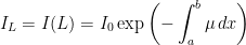
So, given 
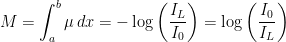
But from
In two dimensions, things change. Given the total absorption for every cross-section through the body, we can construct the absorption coefficient 
The attenuation of an x-ray beam is measured by comparison with the radiation absorbed by water, and is expressed in Houndsfield units, after one of the developers of the CT scanner. Water has a value of 0 Houndsfield units, air is -1000 units and bone is about 1000 units. On an x-ray image, areas with low unit values are black and those with high values are white. Thus, bone shows up as a bright region, the organs are various shades of grey and cavities are black.
The intensity of each x-ray beam gives information about the absorption along a single line through the body. To reconstruct the structure completely, we need x-rays along every line through the body. This is impossible but, from a large set of lines, we can come close to an exact picture.
Any line 


with 

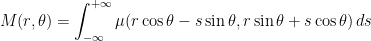
It is this quantity that is measured directly by an x-ray scanner.
The Radon transform is a function of the polar coordinates 

Filtered back projection
How do we recover
The first step is to compute the average of all the line integrals passing through a given point 
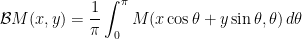
This is called the back projection of 
The link between the Fourier and Radon transforms is expressed by the Central Slice Theorem [Feeman, 2010]. We denote the 1D and 2D Fourier transforms by 


To “undo” the smoothing effect of the back projection, the Radon transform is subjected to a filtering procedure in which high frequencies are boosted. This involves a Fourier transform, followed by multiplication by the (absolute value of) frequency, followed by an inverse Fourier transform. The “filtered back projection” then becomes
![\displaystyle \mu(x,y) = \frac{1}{2} {\cal B} \{ {\cal F}^{-1} [|\omega| {\cal F}({\cal R}\mu)(\omega,\theta) ] \} (x,y)](https://s0.wp.com/latex.php?latex=%5Cdisplaystyle+%5Cmu%28x%2Cy%29+%3D+%5Cfrac%7B1%7D%7B2%7D+%7B%5Ccal+B%7D+%5C%7B+%7B%5Ccal+F%7D%5E%7B-1%7D+%5B%7C%5Comega%7C+%7B%5Ccal+F%7D%28%7B%5Ccal+R%7D%5Cmu%29%28%5Comega%2C%5Ctheta%29+%5D+%5C%7D+%28x%2Cy%29+&bg=ffffff&fg=000000&s=0&c=20201002)
This is the required formula for inversion of the Radon transform.
Here is the recipe: given the Radon transform 
- Take the 1D Fourier transform with respect to the radial variable
- Multiply each component by the absolute value of frequency
- Take the inverse Fourier transform
- Take the back projection.
This leads to the recovery of the original function
Filtered back projection is the fundamental method for reconstruction of the x-ray absorption function. However, it assumes complete knowledge of the Radon transform. In practice, we only have a finite number of x-ray cross-sections. Therefore, only an approximation to the function
Multiplication by 

Further Information
Dean, S. R., 2007: The Radon Transform and some of its Applications. Dover, 295pp. ISBN: 978-0-486-46241-7.
Feeman, T. G., 2010: The Mathematics of Medical Imaging. Springer, 141pp. ISBN: 978-0-387-92711-4.
Radon, J, 1917: On the determination of functions from their integrals along certain manifolds. Translation in [Deans, 2007].
