Waves Packed in Envelopes

In this article we take a look at group velocity and at the extraction of the envelope of a wave packet using the ideas of the Hilbert transform.

Hovmoeller-Arrows

Interference of two waves

A single sinusoidal wave is infinite in extent and periodic in space and time. When waves interact, the dynamics are more interesting. The simplest case is the superposition of two waves. Assume the two components have equal amplitudes and approximately equal wavenumbers and frequencies:

$\displaystyle \psi(x,t) = \cos(k_1x-\omega_1t) + \cos(k_2x-\omega_2t) \,.$

The two components move with phase speeds ${c_1=\omega_1/k_1}$ and ${c_2=\omega_2/k_2}$ . We write the mean values ${\bar k = (k_1+k_2)/2}$ and ${\bar\omega=(\omega_1+\omega_2)/2}$ and the differences ${\Delta k = (k_1-k_2)/2}$ and ${\Delta\omega=(\omega_1-\omega_2)/2}$ . Then by elementary trigonometry we have

$\displaystyle \psi(x,t) = 2 \cos\left(\Delta k\cdot x-\Delta\omega\cdot t\right) \cdot \cos\left(\bar kx-\bar\omega t\right) \,.$

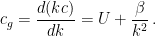
The second factor here (the carrier wave) represents a wave with wavenumber ${\bar k}$ moving with phase speed ${\bar c = \bar\omega/\bar k}$ , close to the phase speeds of the two components. The first factor is slowly varying in space. It is called the envelope, and has wavenumber ${\Delta k}$ and frequency ${\Delta\omega}$ . It moves with a speed ${c_g}$ , called the group velocity,

$\displaystyle c_g = \frac{\Delta\omega}{\Delta k} \,.$

This velocity may be radically different from the phase velocity ${\bar c}$ . More generally, we can write the group velocity as

$\displaystyle c_g = \frac{\partial\omega}{\partial k} = \frac{\partial(kc)}{\partial k} \,.$

Sum of two waves, showing the carrier and envelope.

Group velocity of Rossby waves

Let us look at planetary waves in the atmosphere. For nondivergent quasigeostrophic flow on a beta plane the Rossby wave phase speed is

$\displaystyle c = U - \frac{\beta}{k^2} \,.$

where ${U}$ is the mean zonal flow, ${k}$ is the wavenumber and ${\beta}$ is constant. Because of the minus sign, the phase speed of the waves is westward relative to the mean flow. We compute the group velocity:

$\displaystyle c_g = \frac{d(kc)}{dk} = U + \frac{\beta}{k^2} \,.$

We have the surprising result that the group velocity is directed towards the east (relative to the mean flow), opposite to the phase velocity. The figure below is a Hovmöller diagram, showing the wave amplitude as a function of longitude (horizontal) and time (downward axis). The blue arrow shows the slow progress of an individual wave maximum. The red arrow shows the much faster propagation of the wave group.

Hovmöller diagram, showing wave amplitude as a function of longitude (horizontal) and time (downward axis). Blue arrow: slow progress of an individual wave maximum. Red arrow: rapid propagation of the wave group.

Group velocity is of immense importance in weather forecasting. The large wave-like disturbances in the atmosphere at middle latitudes travel at the phase speed ${c = U - \beta/k^2}$ . But the energy travels at the group velocity ${c_g = U + \beta/k^2}$ , which is often much greater. Wave minima or troughs are commonly linked to stormy weather. Through the action of group velocity, a new storm can appear “spontaneously” downstream of an existing chain of storms. The propagation of energy is more rapid than the movement of the individual storms.

Extraction of the envelope

The envelope of a wave packet may be extracted using ideas based on the Hilbert transform. For full details, see Bracewell (2000, pp. 359-367). Let ${\psi(\xi)}$ be a function on a periodic domain ${0\le\xi<2\pi}$ . We perform the following operations in sequence:

Compute the Fourier coefficients: ${\hat\psi_k= \frac{1}{2\pi}\int_0^{2\pi} e^{-ik\xi} \psi(\xi)\,d\xi}$ .
Set the coefficients to zero for negative index: ${\tilde\psi_k=H_k\hat\psi_k}$ where ${H_k}$ is the Heavyside sequence.
Compute the inverse transform: ${\Psi(\xi)= \sum_{k=0}^{k=\infty} \tilde\psi_k e^{ik\xi}}$ .
Double and take the absolute value: ${A(\xi) = 2|\Psi(\xi)|}$ .

In words, we calculate the Fourier series, throw away the negative frequencies, invert, double and take the absolute value.

A simple example illustrates the technique. Suppose $\psi(\xi)=A\cos n\xi$ . There are just two non-vanishing terms in the Fourier series: $A\cos n\xi = \frac{1}{2} A[\exp(i n\xi)+\exp(-i n\xi)]$ . Elimination of the negative frequency part leaves ${\frac{1}{2} A\exp(in\xi)}$ and twice the absolute value of this is ${A}$ , as expected.

We consider a signal with two wave packets, each with a different carrier frequency and envelope. These are shown in the figure below. The envelope calculated as above is also shown.

WPack3

The envelope extraction may be combined with low-pass or band-pass filtering by replacing the Heavyside function by a suitable masking function, for example

$\displaystyle M(\omega) = \begin{cases} 1, & \omega_{L}\le\omega\le\omega_{H} \\ 0, & \hbox{otherwise} \end{cases}$

which eliminates all components except in the frequency band ${[\omega_{L},\omega_{H}]}$ . We show below the effects of band-passing the signal with wavenubers in the range ${10<k<30}$ (top) and ${30<k<60}$ (bottom), isolating the two packets.

WPack4 WPack5

The Hilbert transform

The theoretical explanation of the envelope extraction method is given in Bracewell (pp. 359-367). The Hilbert transform of a function ${f(t)}$ is defined as

$\displaystyle F(t) = -\frac{1}{\pi}\int_{-\infty}^{+\infty} \frac{f(t^\prime)}{t-t^\prime} dt^\prime$

where the Cauchy principal value of the integral is intended. For a real signal, there is an associated complex signal called the analytical signal, defined by

$\displaystyle f(t) - i F(t) = E(t) \exp(i\omega(t))$

and the amplitude ${E(t)}$ of this signal contains the information about the envelope.

References

Bracewell, R, 2000: The Fourier Transform and its Applications. Third Edn., McGraw-Hill, New York. 636pp.

ThatsMaths