Does Numerical Integration Reflect the Truth?

Many problems in applied mathematics involve the solution of a differential equation. Simple differential equations can be solved analytically: we can find a formula expressing the solution for any value of the independent variable. But most equations are nonlinear and this approach does not work; we must solve the equation by approximate numerical means. The big question is:

“Does the numerical solution resemble the true solution of the equation?”

The answer is: “Not necessarily”.

There are often specific criteria that must be satisfied to ensure that the answer `crunched out’ by the computer is a reasonable approximation to reality. Although the principles of numerical stability are quite general, they are best illustrated by simple examples. We will look at some of these below.

Smooth curve: True solution. Black dots: stable solution. Red dots: unstable solution (time step too large).

The Simplest Cases

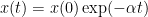
To begin, we take a simple first-order linear ordinary differential equation (ODE):

$\displaystyle \frac{\mathrm{d}x}{\mathrm{d}t} + \alpha x = 0 \,.$

For ${\alpha > 0}$ , the solution ${x(t) = x(0) \exp(-\alpha t)}$ decays exponentially with time. We would expect the numerical solution to do the same. We call this equation the diffusion equation, as it represents a diffusive or damped process.

Let’s discretise the time, replacing a continuous variable by a discrete sequence 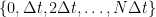${\{ 0, \Delta t, 2\Delta t, \dots, N\Delta t\}}$ , ranging from the initial time to time ${T = N\Delta t}$ . We denote the numerical solution at these times by ${x_n = x(n\Delta t)}$ . For the exact solution we have ${x(n\Delta t) = x(0)\exp(-n \alpha \Delta t)}$ . We may also write this as ${x_n = x_0 \rho^n}$ where ${\rho = \exp(-\alpha\Delta t)}$ . Note that for ${\alpha>0}$ we have ${|\rho|<1}$ , confirming that the solution decreases with ${n}$ .

Euler’s Explicit Method for the Diffusion Equation

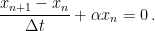
We replace the derivative in the ODE by a finite difference and evaluate the ${\alpha}$ -term at the start of each interval ${[n\Delta t, (n+1)\Delta t]}$ ; this is known as Euler’s method:

$\displaystyle \frac{x_{n+1} - x_n}{\Delta t} + \alpha x_n = 0 \,.$

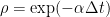
Now seeking a solution of the form ${x_n = x_0 \rho^{n}}$ , we see that we must have

$\displaystyle \rho = 1 - \alpha\Delta t \,.$

For ${\alpha\Delta t < 2}$ , we have ${|\rho| < 1}$ so the solution decays. Moreover, for small values of ${\alpha\Delta t}$ we have ${\rho = 1 - \alpha\Delta t \approx \exp(-\alpha\Delta t)}$ , so that the numerical solution should be close to the true solution, at least for small times. However, if either ${\alpha}$ or the time step is large, we may have ${\alpha\Delta t > 2}$ which means that ${\rho < -1}$ . The numerical solution grows with time and also oscillates between positive and negative values each time step (see illustration above). This solution bears no resemblance to the true (analytical) solution. We see that, for a fixed ${\alpha}$ , a necessary condition for a reasonable solution is that the time step should not be too large:

$\displaystyle \Delta t < \frac{2}{\alpha} \,.$

This is the stability criterion for the Euler forward scheme with the diffusion equation.

An Implicit Method for the Diffusion Equation

Next, we evaluate the ${\alpha}$ -term at the end of the time step:

$\displaystyle \frac{x_{n+1} - x_n}{\Delta t} + \alpha x_{n+1} = 0 \,.$

Then the amplitude ${\rho}$ is given by

$\displaystyle \rho = \frac{1}{1+\alpha\Delta t}$

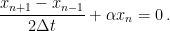
which always has modulus smaller than unity: ${0<|\rho|<1}$ . Consequently, the numerical solution always decays with time and does not oscillate. We say that the implicit method, or backward method, is unconditionally stable.

The Leapfrog Method for the Diffusion Equation

Now for a surprise: we examine the stability of the so-called leapfrog method. Here, the ${\alpha}$ -term is evaluated at the centre of the time step. We might reasonably expect this to yield greater accuracy than either the forward or backward method.

The finite difference equation for the leapfrog method is

$\displaystyle \frac{x_{n+1} - x_{n-1}}{2\Delta t} + \alpha x_{n} = 0 \,.$

Plugging in a solution of the form ${x_n = x_0\rho^n}$ , this yields a quadratic equation for ${\rho}$ :

$\displaystyle \rho^2 + 2 \alpha \Delta t \rho - 1 = 0$

This has two roots,

$\displaystyle \rho_{\pm} = -\alpha\Delta t \pm \sqrt{1 + (\alpha\Delta t)^2}$

It is very clear that the root ${\rho_{-}}$ has modulus greater than 1.

This is unexpected: the leapfrog method is always unstable for the diffusion equation.

The Leapfrog Method for the Wave Equation

The above analysis would suggest that the leapfrog method is useless. However, for some equations it is a very attractive scheme. We consider the simple one-dimensional wave equation

$\displaystyle \frac{\mathrm{d}^2 x}{\mathrm {d}t^2} + \omega^2 x = 0 \,.$

We know that this has an analytical solution ${x(t) = x(0)\sin(\omega t)}$ representing an oscillation or wave-like motion in time. Let us see if this is found for the leapfrog approximation. The ODE is approximated by the finite difference equation

$\displaystyle \frac{x_{n+1} -2 x_n + x_{n-1}}{\Delta t^2} + \omega^2 x_{n} = 0 \,.$

Substituting ${x_n = x_0 \rho^n}$ we get a quadratic equation:

$\displaystyle \rho^2 - (2 - \omega^2\Delta t^2)\rho + 1 = 0$

which has the two roots:

$\displaystyle \rho_{\pm} = (1 - \kappa^2) \pm i \sqrt{\kappa(2-\kappa)}$

where we have written ${\kappa = \omega^2\Delta t^2/2}$ .

It is easy to show that, for ${\kappa<2}$ there are two unimodular roots, that is ${|\rho_{\pm}| = 1}$ , as is the case for the analytical solution. On the other hand, if ${\kappa > 2}$ , there are two real roots, and one of them has a modulus greater than unity. So, the solution blows up.

We conclude that there is a condition for stability of the solution:

$\displaystyle \kappa < 2 \qquad\mbox{or}\qquad \Delta t < \frac{2}{\omega} \,.$

Remarks

CFL-Criterion-Table

The Table above shows the contrasting stability properties of the forward and leapfrog schemes for the two simple equations: the Euler scheme is stable for diffusion and unstable for advection; the Leapfrog scheme is unstable for diffusion and stable for advection. Thus, if we wish to integrate an equation with both processes, we might use one scheme for the diffusion term and another for advection.

The stability criteria have major practical implications. Limitations on the size of the time step mean that more time steps must be taken to reach a given range. In the case of numerical weather prediction, this constrains the delivery time of the computer forecasts.

The first comprehensive analysis of the stability properties of finite difference approximations to differential equations was by Richard Courant, Kurt Friedrichs and Hans Lewy, published in 1928. The constraint on the time step is usually called the CFL criterion. We hope to consider this topic in more detail in a later post.

Sources

The earliest detailed consideration of numerical stability of finite-difference approximations to differential equations is:

${\bullet}$ Courant, R., K. Friedrichs and H. Lewy, 1928: Über die partiellen Differenzengleichungen der mathematischen Physik, Math. Ann., 100 (1), 32-74.

Translation, “On the partial difference equations of mathematical physics”,
IBM J. Res. Dev., 11 (2), 215–234. Available at

https://web.stanford.edu/class/cme324/classics/courant-friedrichs-lewy.pdf

ThatsMaths