Think of a Number: What are the Odds that it is Even?

Pick a positive integer at random. What is the chance of it being 100? What or the odds that it is even? What is the likelihood that it is prime?

EulerProbDist

Probability distribution {P(n)=1/(\zeta(s)n^s)} for s=1.1 (red), s=1.01 (blue) and s=1.001 (black).

Since the set {\mathbb{N}} of natural numbers is infinite, there are difficulties in assigning probabilities to subsets of {\mathbb{N}}. We require the probability of the full set to be unity: {P(\mathbb{N}) = 1}. We also require that the probability function should be additive: {P(A\cup B) = P(A)+P(B)} for disjoint sets {A} and {B}.

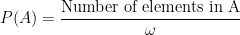
We could try something like

\displaystyle P(A) = \frac{\mbox{Number of elements in A}}{\mbox{Number of elements in N}}

but the denominator — and perhaps also the numerator — is infinite. So, we could try

\displaystyle P(A) = \lim_{n\rightarrow\infty} \left[ \frac {\mbox{Number of elements in A less than n}}{n} \right]

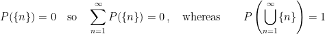
But now the probability for finite sets and, in particular, for any specific number, is zero. So we cannot have additivity:

\displaystyle P(\{n\}) = 0 \quad\mbox{so}\quad \sum_{n=1}^\infty P(\{n\}) = 0 \,, \quad\mbox{whereas}\qquad P\left( \bigcup_{n=1}^\infty \{n\} \right) = 1

Density to the Rescue?

The density of a subset {A} of {\mathbb{N}} can be defined in various ways. If the elements of {A} are arranged in ascending order, we can define

\displaystyle \rho(A) = \lim_{n\rightarrow\infty} \frac{n}{a_n}

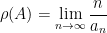
This gives a density of {\textstyle\frac{1}{2}} for the set of even numbers, but it gives a zero density for any finite set. It also gives zero density for many infinite sets, such as the set of squares and the set of prime numbers. So, this will not do.

Another approach is to define probabilities directly, weighting smaller numbers more than larger ones. After all, we may argue that a smaller number is more likely to be chosen in a `random’ selection than a larger one.

We could select a convergent series like {\textstyle{\frac{1}{2} + \frac{1}{4} + \frac{1}{8} + \dots }} that sums to unity and define

\displaystyle P(1) = \frac{1}{ 2} \,, \quad P(2) = \frac{1}{2^2} \,, \quad P(3) = \frac{1}{2^3} \,, \dots \,, P(n) = \frac{1}{2^n} \,, \dots

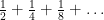
But the chances of an even moderately large number seem unreasonably small: {P(100) = 2^{-100}\approx 10^{-30}}. Moreover, the chances of a randomly chosen number being even or odd are

\displaystyle P(n\ \mbox{even}) = \textstyle{\frac{1}{3}} \qquad P(n\ \mbox{odd}) = \textstyle{\frac{2}{3}}

which hardly gels with our intuition. We need a series that converges much more slowly than the geometric series.

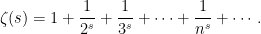
The Euler Zeta-Function

As is well known, the harmonic series diverges:

\displaystyle 1 + \frac{1}{2} + \frac{1}{3} + \dots + \frac{1}{n} + \dots \rightarrow \infty

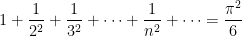
On the other hand, the Basel series converges:

\displaystyle 1 + \frac{1}{2^2} + \frac{1}{3^2} + \dots + \frac{1}{n^2} + \dots = \frac{\pi^2}{6}

If we reduce the index {s} from 2 towards 1, we get a series whose convergence is increasingly slow. It is Euler’s zeta-function, the real case of the Riemann zeta-function:

\displaystyle \zeta(s) = 1 + \frac{1}{2^s} + \frac{1}{3^s} + \cdots + \frac{1}{n^s} + \cdots \,.

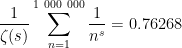
Now we can normalise the series, dividing each term by {\zeta(s)}, and define

\displaystyle P(1) = \frac{1}{\zeta(s)\cdot 1^s} \,, \quad P(2) = \frac{1}{\zeta(s)\cdot 2^s} \,, \quad P(3) = \frac{1}{\zeta(s)\cdot 3^s} \,, \dots \,, P(n) = \frac{1}{\zeta(s)\cdot n^s} \,, \dots

This is well-defined for {s>1}. It allows us to assign a probability to any subset of the natural numbers. Moreover, {\sum P(n) = 1}. Of course, the probability values are sensitive to {s}.

As {s} approaches 1, the distribution becomes increasingly uniform (see Figure at top). For {s=1.1}, the chances of picking a number less than one million are

\displaystyle \frac{1}{\zeta(s)} \sum_{n=1}^{1\ 000\ 000} \frac{1}{n^s} = 0.76268

For {s=1.01}, this is reduced to {P(n<10^6) = 0.13404}. But for infinite sets, things are better. Here are some results for decreasing {s}, calculated with the first million terms

\displaystyle \begin{array}{rcl} s=1.1000 \qquad &P(n\ \mbox{even}) = 0.45699 \qquad &P(n\ \mbox{odd}) = 0.54301 \\ s=1.0100 \qquad &P(n\ \mbox{even}) = 0.47533 \qquad &P(n\ \mbox{odd}) = 0.52467 \\ s=1.0010 \qquad &P(n\ \mbox{even}) = 0.47686 \qquad &P(n\ \mbox{odd}) = 0.52314 \\ s=1.0001 \qquad &P(n\ \mbox{even}) = 0.47701 \qquad &P(n\ \mbox{odd}) = 0.52299 \end{array}

We see that the probabilities for both even and odd numbers are approaching 50%, but the rate of approach is painfully slow. It is possible to use asymptotic results to obtain estimates much more efficiently.

Uniform Probability and Surreals

If we argue that all numbers are `equally likely’, we should choose a uniform distribution. But, since we insist that {P(\mathbb{N})=1}, this works only for a bounded set of numbers:

\displaystyle P(n) = \begin{cases} 1/N, & n\le N \\ 0, & \hbox{otherwise} \end{cases}

We can consider what happens as {N\rightarrow\infty}: then, {P(n) \rightarrow 0} for all {n}.

But what about surreal numbers? Let us return to our initial thought:

\displaystyle P(A) = \frac{\mbox{Number of elements in A}}{\mbox{Number of elements in N}}

The cardinality of {\mathbb{N}} is the surreal number {\omega}, so this is

\displaystyle P(A) = \frac{\mbox{Number of elements in A}}{\omega}

For a singleton, {A = \{n\}}, we have {P(\{n\}) = 1/\omega \equiv \epsilon}. And we have additivity:

\displaystyle P(\mathbb{N}) = P\left( \bigcup_{n=1}^\infty \{n\} \right) = \sum_{n=1}^\infty P(\{n\}) = \omega\epsilon = 1 \,.

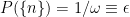
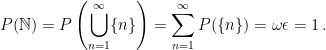
If we now assume that {\omega} is an even number, it follows that

\displaystyle P(n\ \mbox{even}) = \textstyle{\frac{1}{2}} \qquad P(n\ \mbox{odd}) = \textstyle{\frac{1}{2}} \,.

Isn’t that nice!

Sources

{\bullet} Diaconis, Persi and Brian Skyrms, 2018: Ten Great Ideas About Chance. Princeton Univ. Press, 255 pages [See Chapter 5].

{\bullet} The Root of Infinity: it’s Surreal. Post on this blog.


Last 50 Posts

Categories

Archives