Benford’s Law Revisited

{Probability for the first decimal digit ${D_1}$ of a number to take values from 1 to 9.

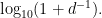
Several researchers have observed that, in a wide variety of collections of numerical data, the leading — or most significant — decimal digits are not uniformly distributed, but conform to a logarithmic distribution. Of the nine possible values, ${D_1=1}$ occurs more than ${30\%}$ of the time while ${D_1=9}$ is found in less than ${5\%}$ of cases (see Figure above). Specifically, the probability distribution is

$\displaystyle \mathsf{P}(D_1 = d) = \log_{10} \left( 1 + \frac{1}{d} \right) \,, \quad \mbox{ for\ } d = 1, 2, \dots , 9 \,. \ \ \ \ \ (1)$

A more complete form of the law gives the probabilities for the second and subsequent digits. A full discussion of Benford’s Law is given in Berger and Hill (2015).

We define the Benford sets ${B_k}$ for ${k=1, 2, \dots , 9}$ as

$\displaystyle B_k = \{n \in\mathbb{N} : D_1(n) = k \} \,.$

The relative density of ${B_k}$ in the range ${[1,n]}$ may be written

$\displaystyle \rho = \frac{\mbox{card}(B_1 \cap \mathrm{N_n})}{n} \,,$

where ${\mathrm{N}_n = \{1, 2, \dots , n \}}$ . This oscillates between ${\frac{1}{9}}$ and ${\frac{5}{9}}$ as ${n}$ increases, and does not approach a limit. In particular, the set ${B_1}$ does not have a natural density. However, we can assign a probability of an arbitrary number being in ${B_1}$ following ideas outlined in Diaconis and Skyrmes (2018) and, in greater detail, in Tenenbaum (1995) [Earlier post: How many numbers begin with a 1?]

Averaging Methods

Different sequences behave differently. The Fibonacci numbers conform to Benford’s Law: the relative frequency of the leading digit ${D_1=d}$ converges to ${\log_{10}(1+{d}^{-1}).}$ The density of the set of Fibonacci numbers that start with ${1}$ is ${\log_{10}2 \approx 0.3010.}$ The sequence of prime numbers does not follow Benford’s Law. For the sequence of natural numbers, the relative density oscillates, with ${\liminf = \frac{1}{9}}$ and ${\limsup = \frac{5}{9}}$ .

For a set ${C\subset\mathbb{N}}$ , the density can be defined as

$\displaystyle \rho_C = \lim_{N\rightarrow\infty} \frac{1}{N} \sum_{n=1}^N \chi_C(n)$

This is an instance of the Cesàro mean, assigning the weight ${1/N}$ to each of the first ${N}$ terms.

There are several alternative ways to specify density. The harmonic density replaces uniform weights ${1/N}$ by the decreasing sequence

$\displaystyle w_n = \left[\frac{1}{H_N}\right]\frac{1}{n} \,,\quad\mbox{where}\quad H_N = \sum_{n=1}^N \frac{1}{n} \,. \ \ \ \ \ (2)$

The numbers ${H_n}$ are known as the harmonic numbers. As is well known, the harmonic series diverges, so ${\lim_{n\rightarrow\infty} H_n = \infty}$ . Diaconis and Skyrmes (2018) describe a generalisation of (2):

$\displaystyle w_n = \left[\frac{1}{\zeta_s(N)}\right]\frac{1}{n^s} \,,\quad\mbox{where}\quad \zeta_s(N) = \sum_{n=1}^N \frac{1}{n^s} \,.$

For ${s>1}$ , the function ${\zeta_s(N)}$ converges to the Riemann zeta-function ${\zeta(s)}$ .

Relative frequency for the first digit of a number to be ${D_1=1}$ (blue) and ${D_1 = 9}$ (red) for ${n}$ between ${1}$ and ${5\times 10^4}$ .

In the Figure above, we show the relative frequency for the first digit of a number to be ${D_1=1}$ (blue curve) and ${D_1 = 9}$ (red curve) for ${n}$ varying from ${1}$ to ${5\times 10^4}$ . This illustrates that, for ${D_1=1}$ , the frequency oscillates between limits of approximately ${\frac{1}{9}}$ and ${\frac{5}{9}}$ .

In the Figure below, we show the relative frequency for the first digit of a number being ${D_1=1}$ , where the logarithmic mean (2) is used. The indication is that the frequency oscillates with reducing amplitude and tends to a limit of approximately 0.3, consistent with Benford’s Law.

{Probability density for ${D_1=1}$ with harmonically weighted probability (2).

The Logarithmic Distribution

We saw that the frequency of occurrence of ${d}$ as the leading digit follows a logarithmic law. But where does this come from? If we assume that all numbers ${n}$ in the range ${1 \le n \le N}$ may occur with equal probability, then the uniform distribution

$\displaystyle \mathsf{P}(n) = \frac{1}{N}$

is appropriate. This leads to the conclusion that all decimal digits should occur with equal probability ${1/9}$ (since zero cannot be a leading digit). However, we could argue that smaller numbers are more probable than larger ones and assign another distribution, such as the logarithmic distribution. We recall that the harmonic numbers are asymptotic to the logarithmic function ${H_n \sim \log n}$ . Thus, to a good approximation, the probability that a randomly chosen number is in the range ${R \le n \le S}$ is ${\log S - \log R = \log S/R}$ .

Now consider a `decade’ of numbers ${10^k \le n \le 10^{k+1}}$ . The probability that a random choice within this interval is ${\log 10^{k+1}-\log 10^k = \log 10}$ , while numbers with leading digit ${1}$ (in the interval ${10^k \le n \le 2\times 10^{k}}$ ) occur with probability ${\log 2\times 10^{k}-\log 10^k = \log 2}$ . Thus, the relative frequency of numbers with leading digit ${1}$ is