A Simple Growth Function

Three Styles of Growth

Early models of population growth represented the number of people as an exponential function of time,

$\displaystyle N(t) = N_0 \exp(t/\tau)$

where ${\tau}$ is the e-folding time. For every period of length ${\tau}$ , the population increases by a factor ${e\approx 2.7}$ . Exponential growth was assumed by Thomas Malthus (1798), and he predicted that the population would exhaust the food supply within a half-century.

Later, the Belgian demographer Pierre François Verhulst refined the model of Malthus, introducing a number called the carrying capacity. This is the maximum population, ${N_\infty}$ , that the environment can sustain. The resulting growth is initially exponential, but flattens out as it approaches the carrying capacity:

$\displaystyle N(t) = \frac{N_\infty}{1+\exp(-t/\tau)}$

This is known as “logistic growth”.

But during the second millennium, each doubling of population took half as long as the previous one. This pattern corresponds to “hyperbolic growth”, with the population increasing beyond all limits within a finite period, much more worrying than exponential growth. A model devised by S von Hoerner predicted that the population would become unbounded by the year 2025:

$\displaystyle N(t) = N_0 \left(\frac{t_\infty}{t_\infty-t}\right)$

This function “blows up”: it is singular as ${t\rightarrow t_\infty}$ . Obviously, such a nightmare scenario would be unsustainable within a short number of years.

$Function {N(t) = N_0 \exp[t/(1+\gamma t)]} for three values of {\gamma}. Blue curve: {\gamma = 0}, exponential growth. Magenta curve: {\gamma = +1}, logistical growth, tending to a finite limit. Red curve: {\gamma = -1}, hyperbolic growth, blowing up at {t=1}.$

Function N(t) = exp[t/(1+g t)]} for three values of g. Blue curve: g = 0, exponential growth. Magenta curve: g = +1, logistical growth, tending to a finite limit. Red curve: g = -1, hyperbolic growth, blowing up at t=1.

A Simple Growth Function

We can illustrate the three styles of growth by means of a single function. Let us consider an exponential function ${N(t) = N_0 \exp(t/\tau)}$ but we now allow the e-folding time to vary linearly with time: ${\tau = \tau_0 + \gamma t}$ . Then we get the function

$\displaystyle N(t) = N_0 \exp\left(\frac{t}{\tau_0+\gamma t}\right)$

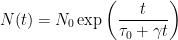
For simplicity we rescale both N and t: ${N -> N/ N_0}$ and ${t->t/\tau_0}$ . Then we obtain a function with just one parameter:

$\displaystyle \mathbf{ N(t) = exp\left(\frac{t}{1+\gamma t}\right) }$

Exponential Growth: If ${\gamma=0}$ , we have exponential growth with e-folding time 1.
Logistic Growth: If ${\gamma>0}$ , the argument of the exponential function tends to ${1/\gamma}$ as ${t}$ becomes large, so the function ${N(t)}$ tends to ${N_\infty = e^{1/\gamma}.}$
Hyperbolic Growth: If ${\gamma<0}$ , the argument of the exponential approaches ${\infty}$ as ${t}$ tends to ${1/| \gamma | }$ and the function has a singularity at this time.