Tap any number into your calculator. Yes, any number at all, plus or minus, big or small. Now tap the cosine button. You will get a number in the range [ -1, +1 ]. Now tap “cos” again and again, and keep tapping it repeatedly (make sure that angles are set to radians and not degrees). The result is a sequence of numbers that converge towards the value 0.739085 … .

What you are calculating is the iterated cosine function
cos ( cos ( cos ( … cos ( x0 ) … ) ) ).
where x0 is the starting value. As the process converges, you have found the solution of the equation
cos( x ) = x
This is called a fixed point of the cosine mapping. If we plot the two functions y = x and y = cos( x ), we see that they intersect in just one point, x=0.739085 … . 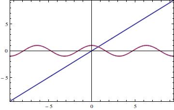 Cobweb Plot We can represent the iterative process of repeating cosine calculations using a diagram called a cobweb plot. On this visual plot, a stable fixed point gives rise to an inward spiral. For a function f ( x ), we plot both the diagonal y = x and the curve y = f ( x ). We are looking for a point where the two graphs cross. Let us start with a point (x0, x0) on the diagonal. For the picture below, we choose ( 0, 0 ). Moving vertically to the curve y = f ( x ), we get the point ( x0, f ( x0 ) ). Now move horizontally to the diagonal again, to ( f ( x0 ), f ( x0 ) ). Moving vertically and horizontally again between the curves, we get (f ( x0 ), f ( f ( x0 ) ) ) and ( f ( f ( x0 ) ), f ( f ( x0 ) ) ). By means of these alternately horizontal and vertical moves, we generate the sequence
{ x0, f ( x0 ), f ( f ( x0 ) ), f ( f ( f ( x0 ) ) ), … }
Under favourable circumstances, the sequence converges to the fixed point of the mapping y = f ( x ). The process is illustrated in the following diagram, starting at ( 0, 0 ) and homing in on the fixed point.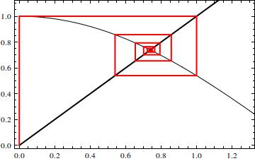 Fixed point theorems (FPTs) give conditions under which a function f ( x ) has a point such that f ( x ) = x. FPTs are useful in many branches of mathematics. Amongst the most important examples are Brouwer’s FPT. This states that for any continuous function f ( x ) mapping a compact convex set into itself, there is a point x0 such that f ( x0 ) = x0. The simplest example is for a continuous function from a closed interval I on the real line to itself. More generally, Brouwer’s theorem holds for continuous functions from a convex compact subset K of Euclidean space to itself. Another FPT is that of Stefan Banach. In technical terms, this states that a contraction mapping on a complete metric space has a unique fixed point.
[Next week: Brouwer’s Fixed Point Theorem]
* * * * * *
 Peter Lynch’s book about walking around the coastal counties of Ireland is now available as an ebook (at a very low price!). For more information and photographs go to http://www.ramblingroundireland.com/
