Random Harmonic Series

We consider the convergence of the random harmonic series

$\displaystyle R = \sum_{n=1}^{\infty}\frac{\sigma_{n}}{n}$

where ${\sigma_n\in\{-1,+1\}}$ is chosen randomly with probability ${1/2}$ of being either plus one or minus one. It follows from the Kolmogorov three-series theorem that the series is “almost surely” convergent.

RandomHarmonicSeriesDistribution

We are all familiar with the harmonic series

$\displaystyle H = 1 + \frac{1}{2} + \frac{1}{3} + \frac{1}{4} + \cdots + \frac{1}{n} + \cdots = \sum_{n=1}^{\infty}\frac{1}{n} \,.$

That it diverges was proved by Nicole Oresme in the fourteenth century and again in the seventeenth century by Pietro Mengoli (who posed the Basel problem; see below), and by both Jakob and Johann Bernoulli.

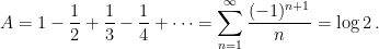
The alternating harmonic series converges:

$\displaystyle A = 1 - \frac{1}{2} + \frac{1}{3} - \frac{1}{4} + \cdots = \sum_{n=1}^{\infty}\frac{(-1)^{n+1}}{n} = \log 2 \,.$

It is a special case of the Taylor series for ${\log(1+x)}$ , first published by Nicholas Mercator (not the cartographer Gerardus Mercator), but discovered independently by Isaac Newton and Gregory Saint-Vincent at about the same time.

Random Harmonic Series

Suppose now that the signs of the terms of the harmonic series ${H}$ are changed in a random manner. We could imagine tossing a coin and choosing plus one for heads and minus one for tails. We get the series

$\displaystyle R = \sum_{n=1}^{\infty}\frac{\sigma_{n}}{n}$

where ${\sigma_n\in\{-1,+1\}}$ is chosen randomly with probability 1/2 of being either plus one or minus one. The series ${R}$ is called a random harmonic series (RHS).

Since there is a likelihood of cancellation between terms of ${R}$ , convergence is a possibility. Indeed, since we expect that “half” the terms are positive and “half” negative, we might expect the RHS to converge, just like the alternating harmonic series ${A}$ .

We may consider ${R}$ to be a random variable. For each choice of the random set ${\{\sigma_n\}}$ it takes a real value or diverges to ${+\infty}$ or ${-\infty}$ . By a symmetry argument, the expected value of ${R}$ is ${E(R)=0}$ . Since ${\sigma_m}$ and ${\sigma_n}$ are uncorrelated for ${m\ne n}$ , the second moment is

$\displaystyle E(R^2) = E\left(\sum_{m=1}^{\infty}\frac{\sigma_{m}}{m} \times \sum_{n=1}^{\infty}\frac{\sigma_{n}}{n}\right) = \sum_{m,n}^{\infty}\frac{E(\sigma_{m}\sigma_{n})} {mn} = \sum_{n=1}^{\infty}\frac{E(\sigma_{n}^2)}{n^2}$

Since ${E(\sigma_{n}^2)=1}$ , this series is the solution of the Basel problem, posed by Pietro Mengoli, and solved by Leonhard Euler in 1734:

$\displaystyle E(R^2) = \sum_{n=1}^{\infty}\frac{1}{n^2} = \frac{\pi^2}{6}$

The sum is the value of the Riemann zeta-function ${\zeta(2)}$ . The standard deviation of ${R}$ is ${\pi/\sqrt{6}\approx 1.28}$ .

With the above properties, it follows from a result of Kolmogorov — the Three-Series Theorem — that a random harmonic series converges almost surely, that is, with probability 1. In contrast, the series

$\displaystyle R = \sum_{n=1}^{\infty}\frac{\sigma_{n}}{\sqrt{n}}$

may be shown, again by means of the Kolmogorov Three-Series Theorem, to diverge.

Riemann’s Rearrangement Theorem

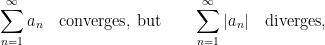
Schmuland (2003) showed that the probability of ${R}$ having a very large value is extremely small, but non-vanishing. There are no upper or lower bounds on ${R}$ so the domain of the distribution is the extended real line ${\bar{\mathbb{R}} = \mathbb{R}\cup\{-\infty,+\infty\}}$ .

This also clear from Riemann’s rearrangement theorem: if an infinite series is conditionally convergent, that is

$\displaystyle \sum_{n=1}^{\infty} a_n \quad\mbox{converges, but}\qquad \sum_{n=1}^{\infty}|a_n|\quad\mbox{diverges,}$

then the terms can be rearranged so that the new series converges to any given real value. Given ${x\in\mathbb{R}}$ , there is a permutation ${\sigma(n)}$ such that

$\displaystyle \sum_{n=1}^{\infty} a_{\sigma(n)} = x \,.$

For simplicity assume ${x>0}$ . We assign ${\sigma(n)=1}$ until the partial sum of ${R}$ exceeds ${x}$ ; then we assign ${\sigma(n)=-1}$ until the partial sum is less than ${x}$ ; and iterate this process so that the sum of the infinite series is ${x}$ . Thus, a random harmonic series (strictly, almost any RHS) can be rearranged to have any real value, or to diverge. But the rearranged series is another RHS.

Numerical Experiments

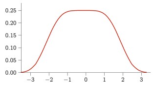
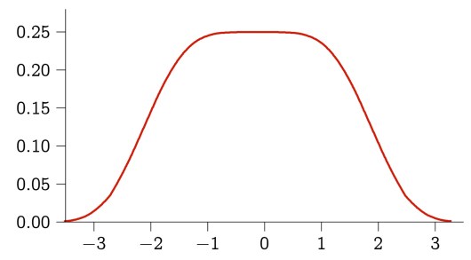
Numerical experiments with large ensembles of random harmonic series show that the sum is generally small. The graph below is the distribution of the random variable ${R}$ . Clearly, it is symmetric about zero, as expected, and falls off sharply for values greater than ${\pm 1}$ . The distribution is very flat near ${R=0}$

Distribution of random variable R (from Schmuland, 2003)

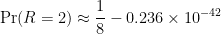
The value of ${\mathrm{Pr}(R=0)}$ looks “suspiciously close to 1/4” (Schmuland, 2003). Also, ${\mathrm{Pr}(R=2)\approx 1/8}$ . Schmuland showed that

$\displaystyle \mathrm{Pr}(R=2) \approx 0.124999999999999999999999999999999999999999764 \dots$

differing from ${1/8}$ by less than ${10^{-42}}$ , an incredibly small quantity

$\displaystyle \mathrm{Pr}(R=2) \approx \frac{1}{8} - 0.236\times 10^{-42}$

Asymmetric series

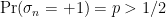
We have assumed that ${\sigma_n}$ takes values ${+1}$ and ${-1}$ with equal probabilities. Suppose now that ${\mathrm{Pr}(\sigma_n=+1)=p>1/2}$ and ${\mathrm{Pr}(\sigma_n=-1)=(1-p)<1/2}$ . The balance between positive and negative terms is now disrupted: there are “more” positive than negative terms. We must therefore suspect divergence of the series. Kolmogorov’s theorem shows this to be the case (MSE, 2015).

Sources

${\bullet}$ Schmuland, Byron, 2003: Random Harmonic Series, Amer. Math. Monthly, 110, 407–416.

${\bullet}$ MSE: Mathematics Stack Exchange (2015).

${\bullet}$ Wikipedia article Harmonic series (mathematics): http://www.wikipedia.org/

ThatsMaths