Geodesics on the Spheroidal Earth – I

Both Quito in Ecuador and Singapore are on the Equator. One can fly due eastward from Singapore and reach Quito in due course. However, this is not the shortest route. The equatorial trans-Pacific route from Singapore to Quito is not a geodesic on Earth! Why not?

A drastically flattened spheroid. Clearly, the equatorial route between the blue and red points is not the shortest path.

The General Equation for Geodesics

Open a typical text on General Relativity. You will probably find a first chapter that is discursive in style, with history and motivation but little or no mathematics. In stark contrast, the second chapter is usually dense with intricate formulae and variables bedecked with subscripts and superscripts. Starting with coordinate transformations, it moves rapidly through tensor algebra to covariant derivatives and culminates with the Riemann curvature tensor ${R^{\sigma}_{\alpha\beta\gamma}}$ .

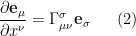
A high point on the route is the equation for the geodesics on a Riemannian manifold

$\displaystyle \frac{d^2 x^\sigma}{d s^2} + \Gamma^{\sigma}_{\mu\nu} \frac{d x^\mu}{d s}\frac{d x^\nu}{d s} = 0 \,. \ \ \ \ \ (1)$

The parameter ${s}$ is the arc-length along the curve. This equation has an austere beauty, but what is it all about? To grapple with it, we need to look at some simple cases. First, we recall Einstein’s summation convention: when the same letter appears as a subscript and superscript, it is assumed to be summed over all the dimensions of the manifold. The ${\Gamma}$ -quantities are the Christoffel symbols. They show how the basis vectors change as we move through space. If the covariant basis is ${\{\mathbf{e}_k\}}$ , then the Christoffel symbols are defined by the equations

$\displaystyle \frac{\partial\mathbf{e}_\mu}{\partial x^\nu} = \Gamma^{\sigma}_{\mu\nu} \mathbf{e}_\sigma \ \ \ \ \ (2)$

The metric tensor, which lies at the basis of the entire geometric structure, is given by ${g_{\mu\nu} = \mathbf{e}_\mu\mathbf{\cdot e}_\nu}$ and the distance element is

$\displaystyle d s^2 = g_{\mu\nu}\,d x^\mu d x^\nu \,.$

Special Cases

The simplest case is for cartesian coordinates. Then the unit orthogonal vectors ${\mathbf{I}}$ and ${\mathbf{J}}$ are constant in space and all Christoffel symbols vanish. Thus ( 1 ) reduces to

$\displaystyle \frac{d^2 x}{d s^2} = 0 \qquad \frac{d^2 y}{d s^2} = 0$

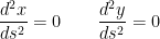
which means that the geodesics are straight lines.

If we transform to polar coordinates ${(r, \theta)}$ , the unit vectors ${\mathbf{e}_r=\mathbf{i}}$ and ${\mathbf{e}_\theta=r\mathbf{j}}$ vary from place to place, and some Christoffel symbols are non-zero. It is elementary — although tedious — to use ( 2 ) to show that

$\displaystyle \Gamma^{\theta}_{r\theta} = \Gamma^{\theta}_{\theta r} = 1/r \,, \qquad \Gamma^{r}_{\theta\theta} = -r$

and all the remaining symbols vanish. Plugging these into (1) we get

$\displaystyle \begin{array}{rcl} \frac{d^2 r}{d s^2} - r \left( \frac{d\theta}{d s}\right)^2 &=& 0 \\ \frac{d^2\theta}{d s^2} + \frac{2}{ r}\frac{d r}{d s} \frac{d\theta}{d s} &=& 0 \end{array}$

It is not immediately obvious how to solve these nonlinear ODEs. We attack the problem from another direction.

Acceleration in Polar Coordinates

We start with the expressions ${x=r\cos\theta}$ and ${y=r\sin\theta}$ relating cartesian and polar coordinates. Differentiating with respect to time we get

$\displaystyle \begin{array}{rcl} \dot x &=& \dot r \cos\theta - r\dot\theta\sin\theta \\ \dot y &=& \dot r \sin\theta + r\dot\theta\cos\theta \end{array}$

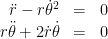
Differentiating again, rearranging and assuming that ${\ddot x = \ddot y = 0}$ , the following equations result:

$\displaystyle \begin{array}{rcl} \ddot r - r \dot\theta^2 &=& 0 \\ r\ddot\theta + 2 \dot r\dot\theta &=& 0 \end{array}$

We see that these are isomorphic to the geodesic equations above, with the arc-length parameter ${s}$ replaced by the time ${t}$ . Since the velocity is constant, this is a legitimate operation. In both cases, the solutions are straight lines in the plane.

Flying along the Equator

We can use the same approach to derive the equations for geodesics on the sphere. Again, three of the eight Christoffel symbols are non-zero. The solutions are the great circles on the sphere. When allowance is made for the oblate form of the Earth, things get more complicated. We will not attempt to write the geodesic equations for a spheroid. However, by looking at the case of extreme flattening, we will see that the shortest route between two points on the spheroid may not be unique.

The equatorial route between the blue and red points is not the shortest path between the two points.

The Figure above shows a spheroid flattened to the extent that it begins to resemble a disk. Looking at the figure, it is clear that the equatorial route from the blue to the red point is not the shortest path between them. There is a shorter route directly across the top of the spheroid. There is a corresponding route across the bottom. These two paths are the geodesics on the spheroid.

Taking things to an extreme, the spheroid collapses to a (two-sided) disk. Then it is obvious that the shortest path between two points on the boundary is along the chord joining them, not along the boundary arc. Since the chord can be on the top or bottom of the disk, the solution is not unique.

Singapore to Quito

These two cities are approximately antipodal to each other. Because of the equatorial bulge, the equatorial route between them is not the shortest route. There are two shortest routes, one north of Hawaii and one south over Australia. We used an online tool for drawing geodesics on Google Maps (reference below) that takes account of the flattening of the Earth. the results are in the Figure below.

Singapore-Quito-Both

Sources

${\bullet}$ Fleisch, Daniel, 2012: A Student’s Guide to Vectors and Tensors. Camb. Univ. Press, 197pp.

${\bullet}$ Karney, CFF. Drawing geodesics on Google Maps [ Website ]

ThatsMaths