Sharp gradients known as fronts form in the atmosphere when variations in the wind field bring warm and cold air into close proximity. Much of our interesting weather is associated with the fronts that form in extratropical depressions.
Below, we describe a simple mechanistic model of frontogenesis, the process by which fronts are formed.
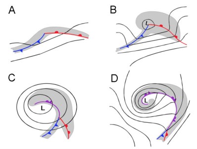
Life-cycle of a Typical Frontal Depression
In the figure below (panel A), the front marks the boundary between polar and tropical airmasses, with cold air advancing southwards and warm air polewards. Images are one day apart. In panel B a clear warm sector has formed, and in panel C the storm is occluding as the cold front overtakes the warm one, forcing the warm air aloft. At four days (panel D) the system is completely occluded.
The Initial Wind and Temperature Fields
A simple model of a storm with frontal formation – a zero-order front – can be constructed, starting from a smooth variation in temperature, shown in the figure below (red denotes warm air and blue denotes cold air). The wind is assumed to blow in a cyclonic circular vortex, as shown in the left-hand panel of the figure.
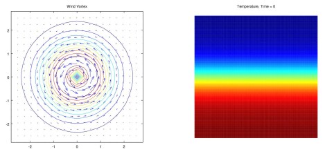
This model is purely kinematic: we suppose that the wind-field does not change in time. However, the temperature changes dramatically as the wind advects and distorts it, bringing warm air northward ahead of the storm and cold air southward behind it.
The motion is a pure rotation with vanishing radial component of velocity and a tangential component varying with distance from the centre:
V = (sech r)2 tanh r
The initial temperature depends only on the north-south direction:
T0 = – tanh y
Development of the Temperature Field in Time.
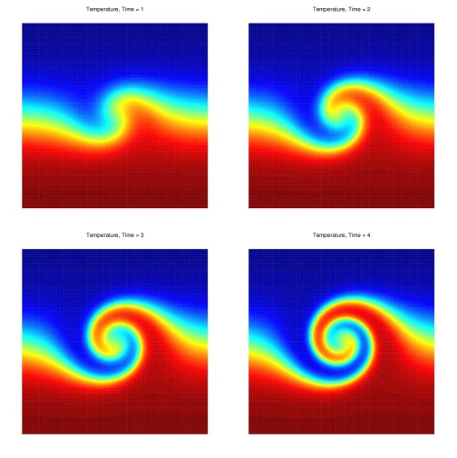
In the figure below, the temperature fields at 1, 2, 3 and 4 days are shown. After one day, a warm front in advance (to the east) of the storm is evident. This sharpens, developing a clear warm sector in the next figure (top right panel). As time proceeds, the front winds up, simulating the occlusion process in a real extra-tropical depression.
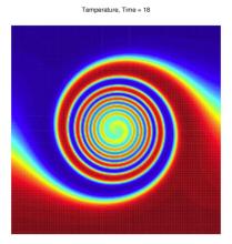
In this simple mechanistic model, the storm continues to “wind up” and extreme gradients develop (see figure at top of post). In the real atmosphere, other processes intervene so that we see structures like those at day 1 and day 2, but not often the extremely tight gradients found in the later images.
The evolving temperature field is obtained by integration of the simple advection equation
d T / d t = 0 .
The analytical solution is easily found: each fluid parcel is carried round a circle with constant angular velocity ω which depends only on the radius. So the value of T(x(t), y(t), t) at time t is equal to its value at a departure point (x0, y0) displaced through an angle ω t :
T(x(t), y(t), t) = T(x0, y0, 0) .
Using this formula, the solution at time t can be found without numerically integrating the equation of motion.
Sources
Doswell, C. A., 1984: A kinematic analysis of frontogenesis associated with a nondivergent vortex. J. Atmos. Sci., 41, 1242–1248.
