Zhukovsky’s Airfoil

A simple transformation with remarkable properties was used by Nikolai Zhukovsky around 1910 to study the flow around aircraft wings. It is defined by

$\displaystyle \omega = \textstyle{\frac{1}{2}}\displaystyle{\left(z +\frac{1}{z}\right)}$

and is usually called the Joukowsky Map. We begin with a discussion of the theory of fluid flow in two dimensions. Readers familiar with 2D potential flow may skip to the section Joukowsky Airfoil.

Visualization of airflow around a Joukowsky airfoil. Image generated using code on this website.

Analytic Functions and Harmonic Functions

Complex variable theory is a powerful tool in modelling fluid flow in two dimensions. The independent complex variable is ${z = x + i y}$ . If a function ${f(z)}$ is analytic, its derivative ${d f/d z}$ does not depend on the direction of the increment ${d z}$ . Therefore

$\displaystyle \frac{\partial f}{\partial x} = \frac{\partial f}{\partial iy}$

Writing ${f(z) = u(x,y) + i v(x,y)}$ , this leads to ${ u_x + i v_x = v_y - i u_y }$ , which immediately yields the Cauchy-Riemann equations:

$\displaystyle u_x = v_y \qquad u_y = - v_x \,.$

It then follows that ${u_{xx} = v_{yx} = v_{xy} = - u_{yy}}$ , so that ${u_{xx} + u_{yy} = 0}$ ; and similarly ${v_{xx} + v_{yy} = 0}$ . Thus, both ${u}$ and ${v}$ satisfy the 2D Laplace equation; they are harmonic functions. This is remarkable: the real and imaginary parts of any analytic function are harmonic functions.

The Complex Potential

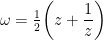
We denote the velocity by ${\mathbf{V} = (u(x,y),v(x,y))}$ . To keep things simple, we will consider steady-state fluid flow ( ${\partial/\partial t = 0}$ ) that is both irrotational and incompressible:

$\displaystyle \delta \equiv \frac{\partial u}{\partial x} + \frac{\partial v}{\partial y} = 0 \qquad\qquad \zeta \equiv \frac{\partial v}{\partial x} - \frac{\partial u}{\partial y} = 0 \,.$

The flow can be represented by a velocity potential ${\phi(x,y)}$ ,

$\displaystyle \mathbf{V} = \boldsymbol{\nabla}\phi \qquad\mbox{so that}\qquad u = \frac{\partial\phi}{\partial x} \mbox{\quad and\quad } v = \phantom{-}\frac{\partial\phi}{\partial y}$

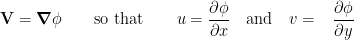
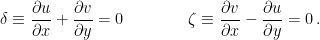
or by a streamfunction ${\psi(x,y)}$ ,

$\displaystyle \mathbf{V} = -\boldsymbol{k\times\nabla}\psi \qquad\mbox{so that}\qquad u = \frac{\partial\psi}{\partial y} \mbox{\quad and\quad } v = -\frac{\partial\psi}{\partial x} \,.$

It follows from ${\delta = \zeta = 0}$ that ${\phi}$ and ${\psi}$ are harmonic functions

$\displaystyle \nabla^2\phi = \phi_{xx}+\phi_{yy} = 0 \qquad \nabla^2\psi = \psi_{xx}+\psi_{yy} =0$

and comprise the real and imaginary parts of an analytical function, the complex potential:

$\displaystyle \omega = \phi + i \psi \qquad\mbox{with}\qquad \frac{\mathrm{d}\omega}{\mathrm{d}z} = u - i v \,.$

Examples of Potential Flow

Example I: The complex potential ${\omega = z}$ corresponds to

$\displaystyle\phi = x \qquad\mbox{and}\qquad \psi = y$

yielding a uniform eastward flow

$\displaystyle u = \phi_x = \psi_y = 1 \qquad\mbox{and}\qquad v = \phi_y = -\psi_x = 0 \,,$

so that ${\mathbf{V} = (1,0)}$ . This is shown in the Figure below (left panel).

Velocity potential ${\phi}$ (dashed blue) and streamfunction ${\psi}$ (solid red) for the complex potentials ${\omega = z}$ (left) and ${\omega =1/z}$ (right).

Example II:
The potential ${\omega = 1/z}$ has velocity potential and streamfunction

$\displaystyle \phi = \frac{x}{x^2+y^2} \qquad\mbox{and}\qquad \psi = \frac{-y}{x^2+y^2}$

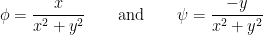
with corresponding velocity components

$\displaystyle u = \frac{x^2-y^2}{(x^2+y^2)^2}\,, \qquad v = -\frac{2xy}{(x^2+y^2)^2} \,.$

This is a dipole flow, shown in the FIgure above (right panel).

Example III: The potential ${\omega = - i\log z}$ can be expressed as

$\displaystyle \omega = - i\log ( r \exp i\theta ) = \theta - i \log r$

and corresponds to velocity potential and streamfunction

$\displaystyle \phi = \theta \qquad\mbox{and}\qquad \psi = - \log r$

with radial and tangential flow components

$\displaystyle v_r = \frac{\partial\phi}{\partial r} = 0 \qquad\mbox{and}\qquad v_\theta = \frac{1}{r}\frac{\partial\phi}{\partial r} = \frac{1}{r}$

which is flow counterclockwise about the origin. Note that the magnitude of ${v_\theta}$ decreases with radius by precisely the amount to ensure

$\displaystyle \zeta = \frac{\partial v_\theta}{\partial r} - \frac{\partial v_r}{\partial \theta} = 0 \,,$

so the flow, although circulating, is irrotational.

The Joukowsky Transform

We combine the complex potentials ${\omega = z}$ and ${\omega = 1/z}$ to produce a potential with some remarkable properties, the Joukowsky potential

$\displaystyle \omega = \frac{1}{2}\left( z + \frac{1}{z} \right) \,.$

This mapping is also called the Zhukovsky transform (Nikolai Zhukovsky studied it around 1910). The velocity potential and streamfunction corresponding to ${\omega}$ are

$\displaystyle \phi(x,y) = \Re\{\omega\} = x + \frac{x}{x^2+y^2} \quad\mbox{and}\quad \psi(x,y) = \Im\{\omega\} = y - \frac{y}{x^2+y^2}$

These functions are plotted below. We note that the unit circle ${|z|=1}$ corresponds to constant ${\psi = 0}$ : there is no flow across this curve and the fluid flows around the unit circle or, in three dimensions, around an infinite cylinder.

Velocity potential ${\phi}$ (dashed blue) and streamfunction ${\psi}$ (solid red) for the complex potential ${\omega = \frac{1}{2}(z+1/z)}$ .

It is obvious from the definition that ${\omega(1/z) = \omega(z)}$ . If we restrict the mapping to the exterior of the unit circle ${|z|=1}$ , it is one-to-one. Rewriting the map as ${z^2 - 2\omega z + 1 = 0}$ , we have two solutions

$\displaystyle z_{+} = \omega + \sqrt{\omega^2-1} \qquad\mbox{and}\qquad z_{-} = \omega - \sqrt{\omega^2-1} \,.$

Since ${z_{+}z_{-}=1}$ , one of these is inside ${|x|=1}$ and the other is outside.

Letting ${z = r\exp(i\theta)}$ the mapping may be written

$\displaystyle \omega = \frac{1}{2}\biggl[r e^{i\theta} + \frac{1}{r}e^{-i\theta}\biggr] = \frac{1}{2}\left[r+\frac{1}{r}\right]\cos\theta + i\frac{1}{2}\left[r-\frac{1}{r}\right]\sin\theta \,.$

Now writing ${\omega = \phi + i\psi}$ we easily show that

$\displaystyle \frac{\phi^2}{a^2} + \frac{\psi^2}{b^2} = 1$

where ${a = \frac{1}{2}(r+1/r)}$ and ${b = \frac{1}{2}(r-1/r)}$ (so ${\omega = a\cos\theta + b\sin\theta}$ ). Thus, circles centered at the origin with ${r>1}$ transform to ellipses
with semi-axes ${a}$ and ${b}$ . Moreover,

$\displaystyle \frac{\phi^2}{\cos^2\theta} - \frac{\psi^2}{\sin^2\theta} = 1$

so lines through the origin are mapped to hyperbolae.

Joukowsky Airfoil

Under the Joukowsky transform, the unit circle maps to the line segment ${\omega \in [-1,+1]}$ (Figure below, left panel). When the centre of the circle is moved to ${z_0}$ but still passes through ${z=1}$ , the image curve represents an airfoil (right panel).

Left: Unit circle maps to line segment. Right: Shifted circle transforms to a curve representing an airfoil.

The mapping that converts a circle into an airfoil also maps the flow around the circle or, in 3D, the cylinder to flow around the airfoil. In the figure below we show a single streamline (left panel) and the corresponding streamline around the airfoil (right panel).

Left: Streamline around cylinder. Right: Corresponding streamline around Airfoil.

Adding Circulation

We saw in Example III above that a potential ${\omega = - i k\log z}$ implies circulation around the wing. This results in lift. In the figure below, the flow without circulation (left panel, ${k=0}$ ) and with circulation (right panel, ${k=0.5}$ ) are shown.

Streamlines around cylinder without circulation (left) and with circulation added to provide lift (right).

A more comprehensive solution for a Joukowsky airfoil is shown in the final figure. This solution was generated using code on the Mathematica StackExchange site referenced below.

Streamlines around a Joukowsky airfoil (see text).

Sources

${\bullet}$ Complex-analysis.com: Website with visualizations: URL

${\bullet}$ Mathematica StackExchange site: URL

${\bullet}$ Spiegel, Murray R., 1964: Schaums Outline Series of Complex Variables. Schaum Publishing Co., New York, 313pp.

${\bullet}$ Strang, Gilbert, 1986: Introduction to Applied Mathematics. Wellesley-Cambridge Press, 758pp. ISBN: 0-961-40880-4.

ThatsMaths