Differential Forms and Stokes’ Theorem

Elie Cartan (1869–1951).

The theory of exterior calculus of differential forms was developed by the influential French mathematician Élie Cartan, who did fundamental work in the theory of differential geometry. Cartan is regarded as one of the great mathematicians of the twentieth century. The exterior calculus generalizes multivariate calculus, and allows us to integrate functions over differentiable manifolds in ${n}$ dimensions.

The fundamental theorem of calculus on manifolds is called Stokes’ Theorem. It is a generalization of the theorem in three dimensions. In essence, it says that the change on the boundary of a region of a manifold is the sum of the changes within the region. We will discuss the basis for the theorem and then the ideas of exterior calculus that allow it to be generalized. Finally, we will use exterior calculus to write Maxwell’s equations in a remarkably compact form.

Stokes’ Theorem

The fundamental theorem of calculus connects differention and integration. For functions defined on the real line ${\mathbb{R}}$ , we have

$\displaystyle \int_{a}^{b} \frac{\mathrm{d}f}{\mathrm{d}x}\,\mathrm{d}x = f(b) - f(a) \,.$

This relates the values of the function ${f(x)}$ on the boundary points of the interval ${[a,b]}$ to the values of the derivative ${\mathrm{d}f(x)/\mathrm{d}x}$ in the interval.

Now suppose ${f(x,y,z)}$ is a function on ${\mathbb{R}^3}$ . Changes in ${f}$ are measured by its gradient, and integrating the gradient along a path ${C}$ from point ${\mathbf{p}_1}$ to ${\mathbf{p}_2}$ , we have

$\displaystyle \int_{C} \boldsymbol{\nabla}f\,\cdot\,\mathrm{d}\boldsymbol{\ell} = f(\mathbf{p}_2)-f(\mathbf{p}_1) \,.$

It follows from this that the integral around a closed curve ${C}$ vanishes:

$\displaystyle \oint_{C}\boldsymbol{\nabla}f\,\cdot\,\mathrm{d}\boldsymbol{\ell} = 0 \,. \ \ \ \ \ (1)$

Moving from a scalar function to a vector field ${\mathbf{P}(x,y,z)}$ , Stokes’ Theorem connects the values of ${\mathbf{P}}$ on the boundary ${\partial S}$ of a 2D surface ${S}$ in ${\mathbb{R}^3}$ to the values of its derivatives in the interior:

$\displaystyle \iint_{S} \mathbf{\nabla\times P\,\cdot\,n} \,\mathrm{d}{\sigma} = \oint_{\partial S} \mathbf{P\,\cdot}\, \mathrm{d}\boldsymbol{\ell} \,. \ \ \ \ \ (2)$

If ${\mathbf{P}=\mathbf{V}}$ is the velocity field, Stokes’ Theorem relates the circulation around the
boundary to the spin, or vorticity, over the surface.

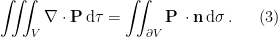
Now considering a 3D volume ${V}$ , the integral of the normal component of a vector field ${\mathbf{P}}$ over its bounding surface is related to the integral of the derivatives of ${\mathbf{P}}$ over the volume by the divergence theorem, or Gauss’s theorem:

$\displaystyle \iiint_{V} \mathbf{\nabla\cdot P}\,\mathrm{d}\mathbf{\tau} = \iint_{\partial V} \mathbf{P\,\cdot n}\,\mathrm{d}\sigma \,. \ \ \ \ \ (3)$

If ${\mathbf{P} = \mathbf{V}}$ is the fluid velocity, this says that the total outward flux through the boundary is equal to the divergence summed over the volume.

There is great similarity between the relationships (1), (2) and (3). They all equate an integral of some differential operator “d” acting on a function ${\omega}$ over a path “ ${C}$ ” (or a higher-dimensional region), to the integral of the function over the the boundary ${\partial C}$ of ${C}$ . We can write all three equations in the form

$\displaystyle \int_C \mathrm{d}\omega = \int_{\partial C} \omega \,. \ \ \ \ \ (4)$

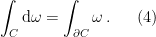
In fact, (4) is the general form of Stokes’ Theorem. Here, ${C \in \Omega}$ is a chain, a combination of ${k}$ -dimensional paths or regions in an ${n}$ -dimensional manifold ${\Omega}$ , with a ${(k-1)}$ -dimensional boundary ${\partial C}$ , and ${\omega}$ is a differential form defined over ${C}$ .

Forms and Chains

A differential form is an expression appearing under an integral sign. The ${k}$ -dimensional forms on an ${n}$ -dimensional manifold ${\Omega}$ comprise a vector space ${\Lambda^k(\Omega)}$ . Cartan defined a multiplication method, the wedge product, which combines elements ${\sigma\in\Lambda^k(\Omega)}$ and ${\tau\in\Lambda^\ell(\Omega)}$ to yield an element ${\sigma\wedge\tau}$ of ${\Lambda^{k+\ell}(\Omega)}$ . The wedge product is skew-symmetric: ${\sigma\wedge\tau = -\tau\wedge\sigma}$ .

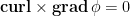
Cartan also defined an operator ${\mathrm{d}\,:\,\Lambda^k(\Omega)\rightarrow\Lambda^{k+1}(\Omega)}$ , called the exterior derivative, which produces a ${(k+1)}$ -form when applied to a ${k}$ -form. If the exterior derivative is applied twice in succession, a null output results: ${\mathrm{d\,d}=0}$ . In the special case ${\Omega=\mathbb{R}^3}$ , it reduces to the classical vector operators grad, curl and div (see table). The familiar identities ${\mathbf{curl\times grad}\,\phi = 0}$ and ${\mathrm{div}\,\mathbf{curl\, V}=0}$ are embraced within the relationship ${\mathrm{d\,d}=0}$ .The differential 0-forms are just real-valued functions on ${\mathbb{R}^3}$ . There are three elementary 1-forms, ${\mathrm{d}x}$ , ${\mathrm{d}y}$ and ${\mathrm{d}z}$ and a general 1-form looks like

$\displaystyle \omega = f_1(x,y,z) \mathrm{d}x + f_2(x,y,z) \mathrm{d}y + f_3(x,y,z) \mathrm{d}z$

There are also just three elementary 2-forms, ${\mathrm{d}x\wedge\mathrm{d}y}$ ${\mathrm{d}y\wedge\mathrm{d}z}$ and ${\mathrm{d}z\wedge\mathrm{d}x}$ and a general 2-form can be written

$\displaystyle \omega = f_1(x,y,z) \mathrm{d}x\wedge\mathrm{d}y + f_2(x,y,z) \mathrm{d}y\wedge\mathrm{d}z$

There are only one elementary 3-form, ${\mathrm{d}x\wedge\mathrm{d}y\wedge\mathrm{d}z}$ and a general 3-form can be written

$\displaystyle \omega = f(x,y,z)\mathrm{d}x\wedge\mathrm{d}y\wedge\mathrm{d}z$

The domain ${C}$ over which differential forms are integrated is called a chain. It may be of any dimension up to that of the underlying manifold. It is inconvenient to restrict the domain to a single connected piece. A ${k}$ -chain is a sum of a finite number of elementary ${k}$ -cells, such as triangles or tetrahedrons, The ${k}$ -chains form a group ${\mathrm{C}_k}$ and the boundary operator reduces the dimension by one: ${\partial\,:\,\mathrm{C}_k\rightarrow \mathrm{C}_{k-1}}$ . Application of the boundary operator twice in succession yields a null result: ${\partial\,\partial\,c = 0}$ .

Application to Maxwell’s Equations

The usual formulation of Maxwell’s equations is in terms of vector operators:

$\displaystyle \begin{array}{rcl} \mathbf{\nabla\times E} = -\frac{\partial\mathbf{B}}{\partial t} \,, &\qquad& \mathbf{\nabla\cdot E} = \rho/\epsilon_0 \,, \\ \mathbf{\nabla\times B} = \frac{1}{c^2}\frac{\partial\mathbf{E}}{\partial t} + \mu_0\mathbf{J} \,, &\qquad& \mathbf{\nabla\cdot B = 0} \,. \end{array}$

This is a system of four vector equations or eight scalar equations. Using differential forms, the system can be written in very compact form. We define a 2-form called the Faraday,

$\displaystyle \mathbf{F} = E_x \mathrm{d}x\wedge\mathrm{d}t + E_y \mathrm{d}y\wedge\mathrm{d}t + E_z \mathrm{d}z\wedge\mathrm{d}t + (B_x\mathrm{d}y\wedge\mathrm{d}z + B_y \mathrm{d}z\wedge\mathrm{d}x + B_z \mathrm{d}x\wedge\mathrm{d}y)$

and the dual 2-form called the Maxwell:

$\displaystyle \mathbf{^*F} = E_x \mathrm{d}y\wedge\mathrm{d}z + E_y \mathrm{d}z\wedge\mathrm{d}x + E_z \mathrm{d}x\wedge\mathrm{d}y - (B_x\mathrm{d}x\wedge\mathrm{d}t + B_y\mathrm{d}y\wedge\mathrm{d}t + B_z\mathrm{d}z\wedge\mathrm{d}t )$

Maxwell’s equations may then be written as

$\displaystyle \mathrm{d}\mathbf{F} = 0 \,, \qquad \mathrm{d}\mathbf{^*F} = \mathbf{^*J} \,. \ \ \ \ \ (5)$

This is clearly a great simplification, at least in formal terms.

A Cautionary Word

There is no doubt that the formalism of exterior calculus provides a powerful toolset for calculus on manifolds. Arnold (1978) is unambiguous in advocating the methods, writing “Hamiltonian mechanics cannot be understood without differential forms”. Of course, a cynic might observe that differential forms were not available to Hamilton!

While the general formalism facilitates the proof of theorems, the development is tortuous, and many definitions are abstract and difficult to visualize. Are difficulties really being removed, or are they being swept under the carpet by the abstract formalism of differential forms? For example, starting from Maxwell’s equations in the form (5), how do we arrive at a wave equation for electromagnetic radiation? (The wave equation follows immediately from the vectorial equations).

In his Lectures on Physics, Richard Feynmann showed how a collection of mathematical or physical equations ${ A_i = B_i}$ can be combined in a single equation

$\displaystyle H = \sum_i (A_i - B_i)^2 = 0 \,.$

Much earlier, in his seminal book Weather Prediction by Numerical Process, Lewis Fry Richardson wrote “There is a tale of a philosopher who succeeded in reducing the whole of physics to a single equation ${H=0}$ , but the explanation of the meaning of ${H}$ occupied twelve fat volumes.” A similar impression may be formed by the student battling with the theory of differential forms. The general form of Stokes’ Theorem (4) does indeed comprise all the familiar integral relationships of classical vector calculus, but it takes a substantial investment of effort to understand what the innocent-looking symbols ${\mathrm{d}}$ and ${\partial}$ actually mean.

Sources

${\bullet}$ Arnold, V. I., 1978: Mathematical Methods of Classical Mechanics. Springer-Verlag, 462p.

${\bullet}$ Flanders, Harley, 1989: Differential Forms with Applications to the Physical Sciences. Dover Publs., New York, 205pp.

${\bullet}$ Richardson, Lewis Fry, 1922: Weather Prediction by Numerical Process. Cambridge Univ. Press. 2nd Edn., 2007. ISBN: 978-0-5216-8044-8 (See page 220).

ThatsMaths