Embedding: Reconstructing Solutions from a Delay Map

In mechanical systems described by a set of differential equations, we normally specify a complete set of initial conditions to determine the motion. In many dynamical systems, some variables may easily be observed whilst others are hidden from view. For example, in astronomy, it is usual that angles between celestial bodies can be measured with high accuracy, while distances to these bodies are much more difficult to find and can be determined only indirectly.

In this article, we pose a general question: can we reconstruct a complete solution of a dynamical problem from a time series of values of a reduced set of variables? In many cases, if a single variable is coupled with the remaining variables through the governing equations, a time series of values of this variable enables us to learn much about the character of the solution. This is done through a process called embedding.

The Idea of Embedding

The state of a physical system may be given by a point in a state space ${S}$ . This may be configuration space, where the coordinates are given as functions if time, or the phase space where coordinates and conjugate momenta are given.

A complete set of initial conditions suffices to determine the motion. But if we cannot observe all the variables, we may be able to make repeated observations of a single variable or a reduced set of variables. An observation is a function ${f:S\rightarrow\mathbb{R}}$ .

Suppose we have a system requiring ${n}$ variables to determine its state. We will assume that the state space ${S}$ is of dimension ${n}$ . If, instead of the ${n}$ independent variables at time ${t_0}$ , we give ${m}$ values of a single variable at ${m}$ times, ${t_1, \dots, t_{m}}$ , we can construct a vector in an ${m}$ -dimensional space ${\mathbb{R}^m}$ : ${(\theta_1, \theta_2, \dots , \theta_m)}$ .

An embedding of a manifold ${S}$ in Euclidean space ${\mathbb{R}^m}$ is a diffeomorphism, a one-to-one differentiable mapping from ${S}$ to ${\mathbb{R}^m}$ with differentiable inverse. A fundamental result in differential topology, due to Hassler Whitney, states that if ${S}$ is a compact manifold of dimension ${n}$ , the set of diffeomorphisms is dense in the space of continuous mappings ${C^1(S,\mathbb{R}^m)}$ provided that ${m>2n}$ . Thus, any such continuous mapping can be approximated with arbitrary precision by an embedding.

In 1981, Dutch mathematician Floris Takens, using the result of Whitney, showed that as long as ${m}$ is sufficiently large relative to ${n}$ , the time series of the variable ${\theta}$ enables us to reconstruct unobserved degrees of freedom. There are several important conditions. For example, the variable ${\theta}$ must be coupled to the other variables through the dynamical equations. The title of Takens’ paper, Detecting Strange Attractors in Turbulence, indicates the focus of his interest. We will examine the Lorenz system — which has a strange attractor — using his ideas; but first let’s consider a much more elementary system, a pendulum.

Delay Map for a Simple Pendulum

Suppose we have a stroboscopic movie of a pendulum. This gives us a sequence of values of the swing-angle at successive moments: ${\{ \theta_1, \theta_2. \dots ,\theta_m\}}$ . We plot ${\sin\theta_n}$ against ${n}$ in the Figure below (left panel). The structure of the solution is not apparent: there are dots everywhere!

Left: Time series of ${\sin\theta_n}$ . Right: Delay plot of ${\sin\theta_{n+3}}$ against ${\sin\theta_n}$ .

Now we use the method of delays: we plot the pairs ${(\sin\theta_n, \sin\theta_{n+d})}$ , where the delay ${d}$ is determined by experiment; in the Figure (right panel), ${d=3}$ . A clear pattern emerges, and all the points are confined to a closed curve, reducing the dimension of the data set. Of course, we know that the sine function is periodic, but this is not evident in the raw data (Figure above, left panel). The delay plot reveals a structure similar to the phase plot where, in ${(\theta,\dot\theta)}$ -space, the trajectory is an ellipse.

A Chaotic System: the Lorenz Equations

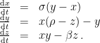
The simple set of three ordinary differential equations introduced by Lorenz in 1963 serves as a valuable example of a chaotic system. These equations have been studied intensively. A 3-dimensional plot of a typical solution is shown at the top of this article. The familiar butterfly-shape is evident.

$\displaystyle \begin{array}{rcl} \frac{\mathrm{d}x}{\mathrm{d}t} &=& \sigma(y-x) \\ \frac{\mathrm{d}y}{\mathrm{d}t} &=& x(\rho-z)-y \\ \frac{\mathrm{d}z}{\mathrm{d}t} &=& xy-\beta z \,. \end{array}$

These three nonlinear equations were derived by Ed Lorenz (1963) to model atmospheric convection. The constants ${\sigma}$ , ${\rho}$ and ${\beta}$ are physical parameters. Lorenz used the values ${\sigma =10}$ , ${\beta =8/3}$ and ${\rho =28}$ ; the system exhibits chaotic behaviour for these values.

We solve the Lorenz equations to get ${(x(t),y(t),z(t))}$ , and in the Figure below (left panel) we plot the component ${x(t)}$ against time. The ${y}$ -component (not shown) behaves in a similar manner. The ${z}$ -component is plotted in the right panel of the Figure. Little understanding of the overall structure of the solution is apparent from these plots except, perhaps, that it looks quite irregular.

Left: Time evolution of ${x(t)}$ . Right: Time evolution of ${z(t)}$ .

The challenge is to find a way of analysing incomplete data, such as a time series of ${x}$ -values, in order to gain a qualitative understanding of the behaviour of the solution. In the Figure below (left panel) we show a plot of ${y(t)}$ versus ${x(t)}$ . This is a projection onto the ${xy}$ -plane of the Lorenz attractor shown at the head of this article.

Left: Plot of ${y(t)}$ versus ${x(t)}$ . Right: Delay plot of ${x(t_{n+6})}$ versus ${x(t_n)}$ .

Now comes a remarkable result: in the right panel of the Figure we show the delay plot of ${x(t_{n+d})}$ versus ${x(t_n)}$ . Although it uses information about only the ${x}$ -component, it is strikingly similar to the the ${xy}$ projection, and shows the characteristic two-leaved structure of the full attractor.

Takens’ result, now called Takens’ Embedding Theorem, shows that the solution of a dynamical system can be reconstructed from a time series of observations. An accessible variable can enable us to recover unobserved degrees of freedom. The trajectory in configuration space and the delay map are structurally similar: they are related through a smooth local coordinate transformation. Thus, it is possible to deduce topologically invariant quantities from the delay map.

Sources

${\bullet}$ Lorenz, E. N., 1963: Deterministic nonperiodic flow. J. Atmos. Sci., 20(2), 130-141.

${\bullet}$ Takens, Floris, 1981: Detecting strange attractors in turbulence. Pp 366-381 in Dynamical Systems and Turbulence, Warwick 1980. Lecture Notes in Mathematics. Springer, Berlin, Heidelberg, ISBN: 978-3-5403-8945-3.

${\bullet}$ Sauer, Timothy D., 2006: Attractor reconstruction. Scholarpedia, 1(10):1727.

* * * * *

That’s Maths II: A Ton of Wonders

by Peter Lynch now available.
Full details and links to suppliers at
http://logicpress.ie/2020-3/

>> Review in The Irish Times <<

* * * *

ThatsMaths