Space-Filling Curves, Part II: Computing the Limit Function

The Approximating Functions

It is simple to define a mapping from the unit interval ${I := [0,1]}$ into the unit square ${Q:=[0,1]\times[0,1]}$ . Georg Cantor found a one-to-one map from ${I}$ onto ${Q}$ , showing that the one-dimensional interval and the two-dimensional square have the same cardinality. Cantor’s map was not continuous, but Giuseppe Peano found a continuous surjection from ${I}$ onto ${Q}$ , that is, a curve that fills the entire unit square. Shortly afterwards, David Hilbert found an even simpler space-filling curve, which we discussed in Part I of this post.

The Hilbert curve is constructed as the limit of a sequence of functions ${H_n(t)}$ from the unit interval ${I=[0,1]}$ to the unit square ${Q = [0,1]^2}$ . The approximating curves give an impression of the Hilbert curve, which we may denote by ${H_\infty}$ or more simply as ${H}$ . However, we did not explain how to calculate the coordinates of the image point ${H(t)}$ for an arbitrary ${t\in I}$ . It was also not obvious that the curve ${H}$ really passes through every point in the unit square.

An Explicit Expression

Hilbert gave a geometrical argument that the function ${H}$ is surjective. However, an explicit expression for ${H}$ was not found for 100 years after Hilbert’s paper appeared. In 1991, Hans Sagan obtained an expression that enables the numerical value of the image of any point to be calculated. For dyadic arguments ${t=k/2^n}$ the expression is a finite sum, yielding an exact answer. For general arguments, the value is given by an infinite sum. The expression is given in Sagan’s book (Sagan, 1994). This book is also an excellent source for more general space-filling curves, covering both the historical development of the subject and the technical details required to construct such curves.

The function ${H : I \rightarrow Q}$

It is convenient to work with quaternary expansions of numbers in the unit interval:

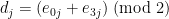
$\displaystyle t = \frac{q_1}{4} + \frac{q_2}{4^2} + \frac{q_3}{4^3} + \cdots \qquad\mbox{where}\qquad q_n\in\{0,1,2,3\} \,.$

As usual, we write ${t = 0.q_1q_2q_3 \dots}$ . Sagan derives the following expression for the image of the point ${t}$

$\displaystyle H(0.q_1q_2q_3 \dots ) = \sum_{j=1}^\infty \frac{(-1)^{e_{0j}}}{2^j}\ \mbox{sgn}(q_j) \begin{pmatrix} (1-d_j)q_j -1 \\ 1 - d_jq_j \end{pmatrix} \ \ \ \ \ (1)$

where ${e_{0 j}}$ is the number of ${0}$ ‘s in ${t}$ preceding ${q_j}$ ( ${\mbox{mod\ } 2}$ ), ${e_{3 j}}$ is the number of ${3}$ ‘s preceding ${q_j}$ ( ${\mbox{mod\ } 2}$ ), ${d_j = ( e_{0j} + e_{3j} )\ (\mbox{mod\ } 2)}$ and ${\mbox{sgn}(q_j)}$ is the signum function of ${q_j}$ .

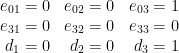
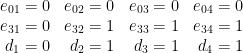
Following Sagan, let us consider a simple example, ${t = \frac{35}{64}}$ , which has the quaternary expansion ${t = 0.203}$ . We easily calculate the following:

$\displaystyle \begin{matrix} e_{01} = 0 & e_{02} = 0 & e_{03} = 1 \\ e_{31} = 0 & e_{32} = 0 & e_{33} = 0 \\ \ d_{ 1} = 0 &\ d_{ 2} = 0 &\ d_{ 3} = 1 \end{matrix}$

Plugging these values into (1) we get

$\displaystyle \begin{array}{rcl} H(0.203) &=& \frac{1}{2}(-1)^0 \begin{pmatrix} (1\cdot 2 - 1) \\ 1 \end{pmatrix} + 0 + \frac{1}{8}(-1)^1 \begin{pmatrix} (0 - 1) \\ 1 - 1\cdot 3 \end{pmatrix} \\ &=& \begin{pmatrix} 1/2 \\ 1/2 \end{pmatrix} + \begin{pmatrix} 1/8 \\ 1/4 \end{pmatrix} = \begin{pmatrix} 5/8 \\ 3/4 \end{pmatrix} \,. \end{array}$

So ${t=0.203 = \frac{35}{64}}$ maps to the point ${(\frac{5}{8},\frac{3}{4})}$ .

We denote the unit square by ${Q = Q_{0}}$ , the first partition into quadrants as ${Q_{10}\cup Q_{11}\cup Q_{12}\cup Q_{13}}$ and so on. Thus, the quadrant ${Q_{ijk} }$ is partitioned into ${Q_{ijk0}\cup Q_{ijk1}\cup Q_{ijk2}\cup Q_{ijk3}}$ . We number the quadrants according to the order in which they come after the reflections required to ensure continuity. Then the point ${(\frac{5}{8},\frac{3}{4})}$ is at the north-east corner of the element ${Q_{203}}$ .

Hilbert Curves in Other Shapes

A continuous function of a continuous function is continuous. Given the space-filling curve ${H(t)}$ on ${Q}$ , we can map ${Q}$ continuously onto another shape and obtain a space-filling curve on that. The shape does not have to be convex, or even simply connected. In the Figure below, we show (approximations to) space-filling curves on the unit square, unit disk, cardioid and annulus.

Approximations to Hilbert curves on a square, disk, cardioid and annulus.

Some Additional Remarks

The Hilbert curve is not just dense in ${Q}$ , but actually passes through every point in the unit square. This is amazing. For all the approximating functions ${H_n(t)}$ , at least one of the coordinates of each point is rational. Therefore, a point such as ${(1/\sqrt{2},1/\pi)}$ cannot be on a curve ${H_n}$ for any ${n}$ . However, since the repeatedly partitioned squares become smaller with each iteration, we can approximate any point ${(x,y)}$ in ${Q}$ by a sequence of squares. Corresponding to these are a nested sequence of diminishing intervals in ${I}$ . Thanks to continuity, the limiting point ${t}$ of this sequence is mapped by the function ${H}$ to the chosen point: ${H(t) = (x,y)}$ .

The construction of ${H(t)}$ ensures its continuity. However, the Hilbert curve is nowhere differentiable. Since Netto proved that one-to-one functions from ${I}$ to ${Q}$ cannot be continuous, the Hilbert curve cannot be injective: it maps ${I}$ onto the entirety of ${Q}$ , but there are many points in ${Q}$ that have more than one pre-image. The central point ${(\frac{1}{2},\frac{1}{2})}$ is one of these.

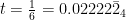
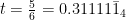
We can approach the central point in several ways. We can jump directly to ${(\frac{1}{2},\frac{1}{2})}$ , which is what happens for the quaternary expansion of ${t=\frac{1}{2}}$ , which is ${0.20000\bar{0}}$ . We can also get there by choosing the quadrant ${Q_{10}}$ and then the north-east quadrant at each subsequent scale. This happens for the number ${0.02222\bar{2}}$ , which corresponds to ${t = \frac{1}{6}}$ . Finally, we can get to the centre by choosing ${Q_{03}}$ and then the north-west quadrant at all smaller scales, which arises from the number ${0.31111\bar{1}}$ or ${t=\frac{5}{6}}$ . Thus, all the points ${\{\frac{1}{6},\frac{1}{2},\frac{5}{6}\}}$ in the unit interval ${I}$ map to the same point in ${Q}$ .

“But yet I’ll make assurance double sure”

Let us confirm that (1) gives the correct results. For ${t = \frac{1}{2}=0.2_4}$ , the expansion reduces to a single term ${(1/2,1/2)}$ .

For ${t=\frac{1}{6} = 0.02222\bar{2}_4}$ we have

$\displaystyle \begin{matrix} e_{01} = 0 & e_{02} = 1 & e_{03} = 1 & e_{04} = 1 \\ e_{31} = 0 & e_{32} = 0 & e_{33} = 0 & e_{34} = 0 \\ \ d_{ 1} = 0 &\ d_{ 2} = 1 &\ d_{ 3} = 1 &\ d_{ 4} = 1 \end{matrix}$

and the expansion is

$\displaystyle 0 + \frac{1}{4}(-1)^1 \begin{pmatrix} -1 \\ -1 \end{pmatrix} + \frac{1}{8}(-1)^1 \begin{pmatrix} -1 \\ -1 \end{pmatrix} + \cdots = \begin{pmatrix} {\frac{1}{4}+\frac{1}{8}+\frac{1}{16} \cdots} \\ [\frac{1}{4}+\frac{1}{8}+\frac{1}{16} \cdots] \end{pmatrix} = \begin{pmatrix} 1/2 \\ 1/2 \end{pmatrix} \,.$

For ${t = \frac{5}{6}=0.31111\bar{1}_4}$ , we get

$\displaystyle \begin{matrix} e_{01} = 0 & e_{02} = 0 & e_{03} = 0 & e_{04} = 0 \\ e_{31} = 0 & e_{32} = 1 & e_{33} = 1 & e_{34} = 1 \\ \ d_{ 1} = 0 &\ d_{ 2} = 1 &\ d_{ 3} = 1 &\ d_{ 4} = 1 \end{matrix}$

and the expansion is

$\displaystyle \frac{1}{2} (-1)^0 \begin{pmatrix} 1\cdot 3-1 \\ 1-0 \end{pmatrix} + \frac{1}{4}(-1)^1 \begin{pmatrix} -1 \\ 0 \end{pmatrix} + \frac{1}{8}(-1)^1 \begin{pmatrix} -1 \\ 0 \end{pmatrix} + \cdots \\ = \begin{pmatrix} 1 - \frac{1}{4}[1+\frac{1}{2}+\frac{1}{4} \cdots] \\ 1/2 \end{pmatrix} = \begin{pmatrix} 1/2 \\ 1/2 \end{pmatrix} \,.$

Thus, all three values of ${t}$ map to the central point of the unit square.

Some beautiful animations of the Hilbert curve are given on Brian Hayes’ website. See also his book (Hayes, 2017).

Sources

${\bullet}$ Hayes, Brian, 2017: Foolproof, and Other Mathematical Meditations. MIT Press. 248pp. ISBN: 978-0-2620-3686-3.

${\bullet}$ Sagan, Hans, 1994: Space-filling curves. Springer-Verlag, New York. 193pp. ISBN: 0-387-94265-3.

ThatsMaths