Spiric curves and phase portraits

Left: Conic sections. Right: Spiric sections [images Wikipedia Commons].

We are very familiar with the conic sections, the curves formed from the intersection of a plane with a cone. There is another family of curves, the Spiric sections, formed by the intersections of a torus by planes parallel to its axis. Like the conics, they come in various forms, depending upon the distance of the plane from the axis of the torus (see Figure above). We examine how spiric curves may be found in the phase-space of a dynamical system.

Coordinates on the Torus

A torus (Greek ${\mathit{\sigma\pi\epsilon\iota\rho\alpha}}$ , torus) may be considered as a product of two circles, ${S^{1}\times S^{1}}$ . Spiric sections are the intersections of planes parallel to the axis of the torus. The position on a torus may be specified by toroidal and poloidal coordinates. The toroidal component ( ${\lambda}$ ) is the angle following a large circle around the torus. It is analogous to the longitude, varying along the parallels. The poloidal coordinate ( ${\theta}$ ) varies along a smaller circle around the surface; changing ${\theta}$ is like altering the latitude. Both parameters take all values in the range ${[0,2\pi)}$ .

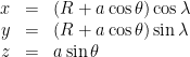
The equations in cartesian coordinates for a point on the torus with toroidal/poloidal coordinates ${(\lambda,\theta)}$ are given by

$\displaystyle \begin{array}{rcl} x &=& (R + a \cos\theta )\cos\lambda \\ y &=& (R + a \cos\theta )\sin\lambda \\ z &=& a \sin\theta \end{array}$

(we assume ${a<R}$ ). Suppose we take the plane ${y=y_0}$ or — using the parametric equations — ${(R + a\cos\theta)\sin\lambda=y_0}$ . Substituting this into the other equations, we get a quartic relationship between ${x}$ and ${z}$ :

$\displaystyle [(x^2+z^2)-(R^2+a^2-y_0^2)]^2 = 4R^2(a^2-z^2) \,.$

These curves are known as the spiric sections of Perseus. Almost nothing is known about Perseus, except that he was active in the second century BC. Proclus (AD 411–485) wrote that Perseus is associated with the spiric curves in the same way as Apollonius is linked to the conics. Spiric sections include the ovals of Cassini as special cases. A set of such curves is shown in the Figure below.

Spiric sections: intersections between a torus and a plane parallel to its axis.

In the Figure below, we plot spiric curves for intercept values in the range ${y_0\in\{0.0,0.9,1.0,1.1,1.3,2.0,2.5,2.95\}}$ , with parameter values ${R=2}$ and ${a=1}$ . In the limiting case ${y_0=0}$ , the spiric is comprised of two circles. As ${y_0}$ increases, these are distorted and when ${y_0=1.0}$ , they merge into a single curve, the lemniscate of Bernoulli. As ${y_0}$ grows further, this becomes peanut-shaped and then a convex oval before reducing to a point when ${y_0 = 3}$ .

Spiric curves for parameter values ${y_0\in\{0.0,0.9,1.0,1.1,1.3,2.0,2.5,2.95\}}$ .

Another Perspective

It is enlightening to plot the spirics as functions of the toroidal and poloidal coordinates. We do this in the following figure. The image is symmetric about the vertical through ${\lambda=\pi}$ . The two curves corresponding to the lemniscates are plotted in red.

Spiric curves in ( ${\lambda,\theta}$ )-space, for ${y_0\in\{ 0.0, 0.25, 0.5, 1.0, 1.5, 2.0, 2.5, 2.95 \}}$ .

Left: Spiric curves in ( ${\lambda,\theta}$ )-space, for ${y_0\in\{ 0.0, 0.25, 0.5, 1.0, 1.5, 2.0, 2.5, 2.95 \}}$ . Right: phase plane for a simple pendulum.

In the above figure, we switch the coordinates ${\lambda}$ and ${\theta}$ (left panel). In the right panel we show the phase portrait for a simple pendulum. The similarity between the two plots is clear. For the pendulum, each curve represents a specific energy level. As energy is conserved, the trajectories in phase space lie on constant energy surfaces.

Left: Phase plane wrapped into a cylinder. Right: Cylinder bent around into a tube. Curve heights correspond to energy [Figures from Stewart (1997)].

A clever representation of the motion, with energy as the vertical coordinate, was discussed in Ian Stewart’s book Does God Play Dice? In the figure above, the phase plot of the simple pendulum is curled around into a cylinder (left panel) and this cylinder is then bent around into a U-shaped surface (right panel). In the right panel, the trajectories are found at fixed vertical levels (fixed energies). We can see how these curves appear similar to the spiric section curves plotted above.

It would be interesting to consider the nature of a dynamical system whose trajectories are spiric curves.

Sources

${\bullet}$ Stewart, Ian, 1997: Does God Play Dice? The New Mathematics of Chaos. Penguin UK. ISBN: 9780141928074.

${\bullet}$ Wikipedia article Spiric section: Wiki

ThatsMaths