Poincaré’s Half-plane Model

For two millennia, Euclid’s geometry held sway. However, his fifth axiom, the parallel postulate, somehow wrankled: it was not natural, obvious nor comfortable like the other four.

In the first half of the nineteenth century, three mathematicians, Bolyai, Lobachevesky and Gauss, independently of each other, developed a form of geometry in which the parallel postulate no longer applied. This later bacame known as hyperbolic geometry.

A model context in which the axioms of hyperbolic geometry held was devised by Eugenio Beltrami. This demonstrated the internal consistency of the new geometry.

Henri Poincaré studied two models of hyperbolic geometry, one based on the open unit disk, the other on the upper half-plane. The half-plane model comprises the upper half plane ${H = \{(x,y): y>0\}}$ together with a metric

$\displaystyle d s^2 = \frac { d x^2 + d y^2 } { y^2 } \,.$

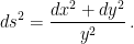
It is remarkable that the entire structure of the space follows from the metric, although not without some effort.

Metric and Geodesics

What are the “straight lines” in this model? For two points ${P}$ and ${Q}$ in ${H}$ , the distance between them is

$\displaystyle s = \int_P^Q \, d s = \int_P^Q L(y,y^\prime) \, dx$

where ${y^\prime = dy/dx}$ and ${L(y,y^\prime) = \sqrt{(1+{y^\prime}^2)/y^2 }}$ may be called the Lagrangian. We can write down the Euler-Lagrange equation for the solution that minimises this distance, and it is

$\displaystyle y y^{\prime\prime} + ( 1+{y^\prime}^2 ) = 0 \,.$

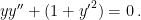
This is the equation for the geodesics ${y(x)}$ .

How to Solve the Geodesic Equation

One way to find the solution is to look it up in a dusty old book like Kamke [K48], where the equation is found on page 573 (§6.126). The solutions are described as Halbkreise, or semicircles. Thus, the geodesics in ${H}$ are the semicircles

$\displaystyle y = \sqrt{ a^2 - (x-x_0)^2}$

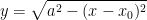
with centre at ${(x_0,0)}$ and radius ${a}$ . Thank you very much, Herr Dr. Kamke.

Some of these semcircles are shown in the figure below.

Geodesics in the Poincare Half-plane

Why Hyperbolic Geometry?

Geometries with constant curvature fall into three categories, elliptic with positive curvature, Euclidean or flat with zero curvature and hyperbolic with negative curvature.

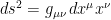
We can compute the curvature of the half-plane ${(H,ds)}$ . The details are many, and we shall show only the main steps (for details, see [L13]). We write the metric, with the usual summation convention, as

$\displaystyle ds^2 = g_{\mu\nu} \, dx^{\mu} x^{\nu}$

where

$\displaystyle g_{\mu\nu} = \begin{pmatrix} 1/y^2 & 0 \\ 0 & 1/y^2 \end{pmatrix}$

The Christoffel symbols of the first and second kind can be computed. There are eight of each kind but, for the half-plane, many of them are zero. Knowing them, we can compute the Riemann curvature tensor:

$\displaystyle R^{\sigma}_{\ \alpha\beta\gamma} = \frac{\partial\Gamma_{\alpha\gamma}^\sigma}{\partial x^\beta} - \frac{\partial\Gamma_{\beta\gamma}^\sigma}{\partial x^\alpha} + \Gamma_{\alpha\gamma}^\tau \Gamma_{\tau\beta}^\sigma - \Gamma_{\alpha\beta}^\tau \Gamma_{\tau\gamma}^\sigma$

There are 16 components in this tensor but most of them vanish, and we are left with just

$\displaystyle R^{1}_{\ 212} = - R^{1}_{\ 221} = R^{2}_{\ 121} = - R^{2}_{\ 112} = - 1/y^2$

In fully covariant form, the non-zero components are

$\displaystyle R_{1212} = R_{2121} = - 1/y^4 \qquad R_{1221} = R_{2112} = + 1/y^4$

Defining ${g=\det(g_{\mu\nu})}$ , we can write the Gaussian curvature in terms of an element of the Riemann tensor:

$\displaystyle \kappa = R_{1212} / g = -1 \,.$

Thus, the half-plane model has uniform negative curvature and is a hyperbolic space.

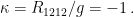
An Easier Way to See Hyperbolicity

We can see from the figure of the half-plane, and the knowledge that the geodesics are semicircles with centres on the ${x}$ -axis, that for a given “straight line” and a point not on it, there is more than one line that does not intersect the given line. That is, many lines can be drawn through the point that are parallel to the given line. An example is given in the figure below: both thin lines through ${P}$ are parallel to the thick line L. In fact, there are an infinite number of such lines.

Both lines through P are parallel to the heavy line L. There are an infinite number of such lines through P parallel to L.

Sources

[K48] Kamke, E., 1948: Differentialgleichungen: Lösungsmethoden und Lösungen. Band 1. Gewönliche Differentialgleichungen. 3rd Edn., Chelsea Publ., New York. 666pp.

[L13] Lynch, P, 2013: Curvature of the Poincaré Half-Plane. ( PDF )

ThatsMaths