The powerful and versatile computational software program called Mathematica is widely used in science, engineering and mathematics. There is a related system called Wolfram Alpha, a computational knowledge engine, that can do Mathematica calculations and that runs on an iPad.

Mathematica can do numerical and symbolic calculations. Algebraic manipulations, differential equations and integrals are simple, and a huge range of beautiful graphs can be plotted in an instant.
Searching in Wolfram Alpha, I found some graphs called “heart curves”, one of which is plotted here:
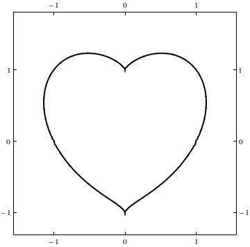 This Heart Curve has the equation
(x² + y² – 1)³ – x² y³ = 0.
Bonne’s Projection and the Werner Projection
Heart-shaped curves arise in some applications. One such is the Werner Projection, a special case of Bonne’s Projection:
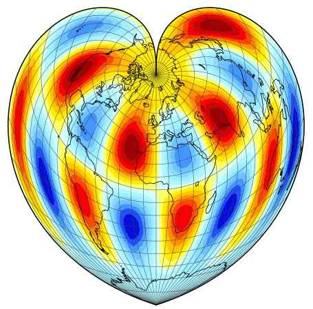
This plot was made with the free software package called Panoply.
Variations on the Heart Curve
The algebraic form of the Heart Curve is a sixth order polynomial in x and y. Note that, as only even powers of x occur, the curve has bilateral symmetry, a property found in the bodies of many animals and, of course, in the human face.
The equation can be written in polar coordinates,
(r² – 1)³ – (r cos φ)³ (r sin φ)² = 0
where the angle φ is measured from the vertical or y axis. This also shows the bilateral symmetry, as the trigonometric function is an even function of φ.
If, on the right hand side of the above equation, 0 is replaced by a parameter α, the character of the curve changes as the value of α changes. The function Manipulate in Mathematica allows one to explore the effect of a changing parameter: as the value is varied by means of a slider, the displayed graph changes too.
In the case of the curve defined by
(x² + y² – 1)³ – x² y³ = α
the graph changes gradually from the Heart Curve to a circle as α increases to larger positive values. However, as α becomes more negative the curve changes in more interesting ways. It develops lobes at the top left and right and eventually, at about α = –0.1, these break off into separate closed curves. For α < – 1.0 there are no real points on the curve and the plot is empty.
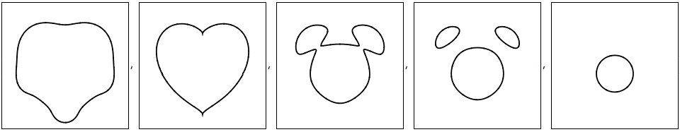
Yogi Bear Curve
A nice “fun curve” results for α = – 0.1 when the lobes have developed to look like the ears of a cartoon character (see middle plot above). In the plot at the top of this article, we combine two curves, one with α = – 0.1 for the outline and one with α = – 0.2, but scaled down to half size, for the eyes and nose. In fact, this “Yogi Bear Curve” can be generated with a single command in Mathematica:
ContourPlot[((x^2 + y^2 – 1)^3 – x^2 y^3 + 0.1) * (((2 x)^2 + (2 y)^2 – 1)^3 – (2 x)^2 *(2 y)^3 + 0.2),{x, -1.5, +1.5}, {y, -1.25, +1.75}, Contours -> {0}, ContourShading -> True, ContourStyle -> Thickness[0.01],FrameTicks -> False, Axes -> None, Frame -> False,ImageSize -> Large]
This is just the zero-contour of a product of two sixth-order polynomials.
You can have fun designing curves to represent your favourite cartoon characters. It should not be difficult to modify the Yogi Bear Curve to make it look like Mickey Mouse. Mathematica is not essential. Free software packages like Octave are fine too.
* * * * * *

Peter Lynch’s book about walking around the coastal counties of Ireland is now available as an ebook (at a very low price!). For more information and photographs go to http://www.ramblingroundireland.com/
