Curves with Singularities

Many of the curves that we study are smooth, with a well-defined tangent at every point. Points where the derivative is defined — where there is a definite slope — are called regular points. However, many curves also have exceptional points, called singularities. If the derivative is not defined at a point, or if it does not have a unique value there, the point is singular.

Slinky traces a smooth helical curve in three dimensions.

Generally, if we zoom in close to a point on a curve, the curve looks increasingly like a straight line. However, at a singularity, it may look like two lines crossing or like two lines whose slopes converge as the resolution increases.

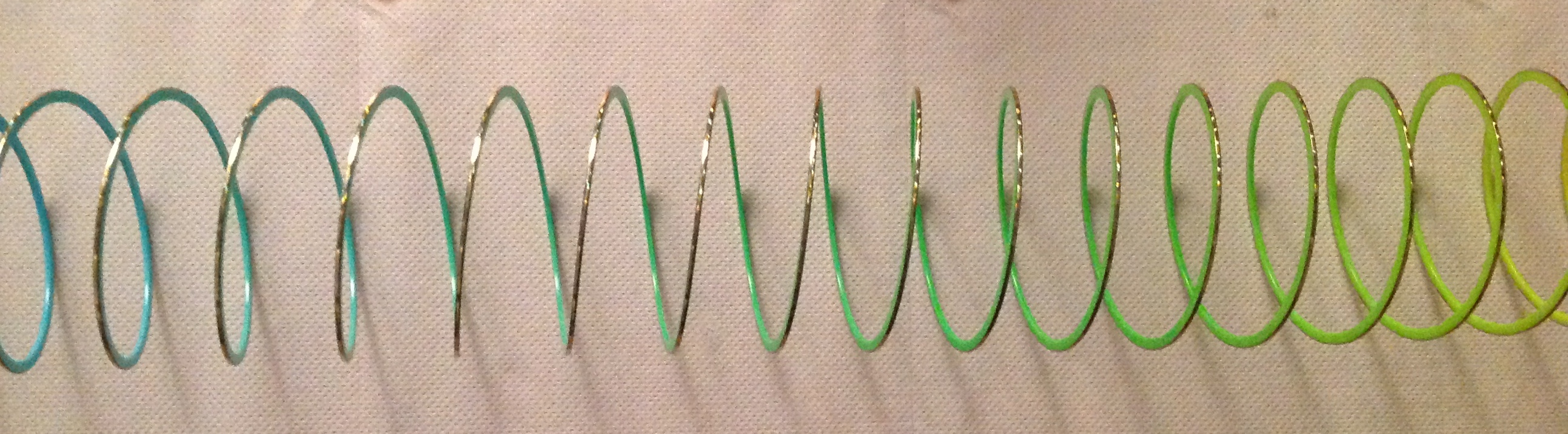
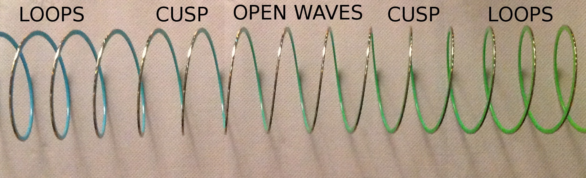
Projection of a Helix

By treating a two-dimensional curve as the projection, or shadow, of a curve in space, we can view a singularity as an artifice of perspective, a kind of optical illusion.The figure above shows a slinky stretched out on a table. It traces a smooth helical curve in three dimensions. However, its projection onto two dimensions gives rise to exceptional points. These may be cusps, where the projected curve suddenly changes direction, or loops where it crosses itself, as shown here:

Projection of slinky onto two dimensions has singular points.

In general, smooth curves can acquire singularities through projection from 3D space to a 2D plane. Think of a piece of string dropped on the floor: while the projection crosses itself and so has singular points, the actual string in three dimensions does not intersect itself. It is generic for smooth manifolds to acquire singularities through the process of projection. Reversing the process, the singularities may be removed by embedding the curve in a higher dimensional space.

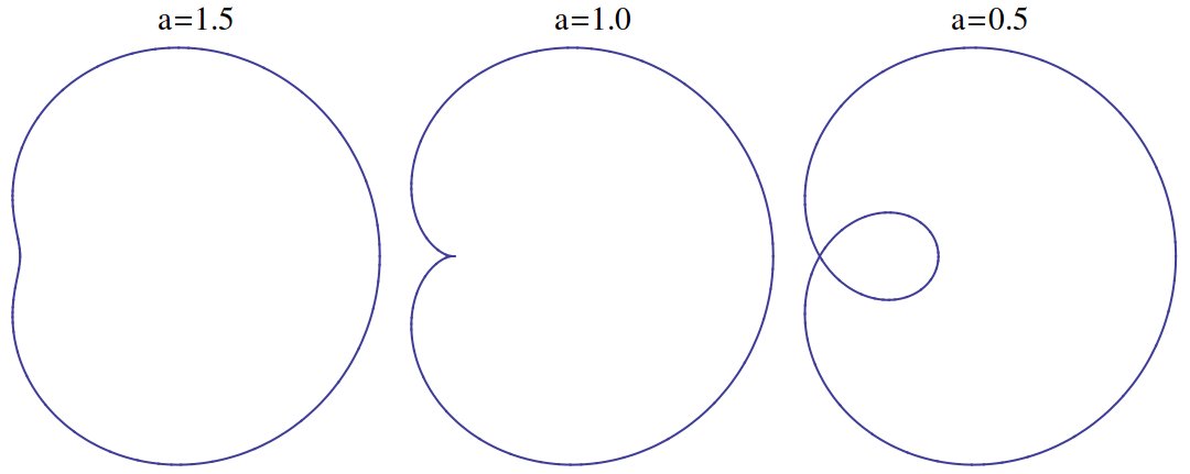
As another example, the next figure shows graphs of the limacon curve ${r=a+\cos\theta}$ for ${a\in\{1.5,1.0,0.5\}}$ . For a > 1, the curve is smooth. For a = 1, it is a cardioid, with a cusp at the origin. When a < 1, the curve crosses itself at the origin.

$Three lima\c{c}ons illustrating double points. Left: Smooth curve {r=1.5+\cos\theta}. Centre: Cardioid {r=1.0+\cos\theta} with a a cusp at the origin. Right: Curve {r=0.5+\cos\theta} crosses itself at the origin$

Three limacons. Left: Smooth curve with a = 1.5. Centre: Cardioid (a = 1.0) with a cusp at the origin. Right: Curve with a = 0.5 crosses itself at the origin.

Singular Points on Cubic Curves

We can specify a curve in the (x, y)-plane in several ways: by a function ${y = f(x)}$ or implicitly as ${F(x,y)=0}$ or parametrically, ${\{(x(t),y(t)): t\in[a,b]\}}$ . If the function ${F(x,y)}$ is linear in both arguments, it specifies a straight line. If it is quadratic, it describes a conic section.

Conics have been studied since ancient times and Apollonius identified three species, the ellipse, parabola and hyperbola. Generically, all these curves are smooth: they have well-defined tangents at all points.

Curves with cubic dependency on the arguments were first analysed by Isaac Newton; there are 78 different cases to consider. These cubic curves exhibit a new phenomenon: they can have singularities in the form of cusps, or they can cross themselves with more than one tangent line at a single point.

As examples of simple cubic curves, let us consider the two curves

$\displaystyle y^2 = x^3 \qquad\mbox{and}\qquad y^2 = x^3 + x \,.$

These are graphed in the figure below.

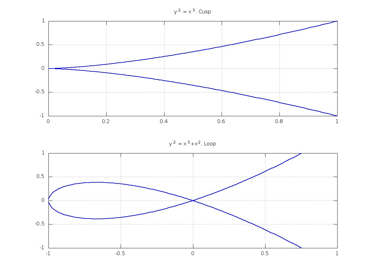
Top: Cusp in function y^2 = x^3. Bottom: Loop in function y^2 = x^3 + x^2.

We see that the curve ${y^2 = x^3}$ , known as a semi-cubic parabola, has a cusp, coming to a point at the origin. If we zoom in to this point, the curve fails to resemble a line segment but looks like two line segments terminating at the origin. This is the cusp singularity.

The function ${y^2 = x^3 + x}$ has a double point at the origin. Zooming in, it resembles two lines crossing, and the tangent is not uniquely defined.

Removing Singularities
There are ways to transform a curve so as to remove singularities, but this must be done so as not to lose information about the original curve. For one-dimensional curves, it is always possible to carry out this process, called regularisation or resolution of the singularity. For higher-dimensional shapes, surfaces, volumes and so on, it is not so straightforward.

The mathematician Oscar Zariski studied singularities in two and three dimensions. In 1970, his student Heisuke Hironaka won a Fields Medal for showing that singularities in shapes of every dimension can be resolved. Thus, a polynomial equation of arbitrary degree in any number of variables is equivalent to one that is regular, that is, free from singularities.

In the physical world, we find singularities in many contexts. A frequently cited example is a black hole, a gravitational singularity at the heart of a galaxy. Less exotic but equally valid examples are the flickering patterns of sunlight on the bottom of a swimming pool when the water is rippled. Even closer to home, optical caustics show up on the surface of a cup of coffee.

Optical caustic on the liquid surface of a cup of coffee. A cusp can be seen in the cardioid curve.

Optical caustic in a coffee cup. A cusp can be seen in the cardioid curve.

Sources

♦ Elwes, Richard, 2013: Maths in 100 Key Breakthroughs. 416pp. ISBN: 9-781-780-87322-0.

♦ Wikipedia article: Singular Points on Curves.

♦ Wikipedia article: Singularity Theory.

ThatsMaths