Bent Coins: What are the Odds?

If we toss a `fair’ coin, one for which heads and tails are equally likely, a large number of times, we expect approximately equal numbers of heads and tails. But what is `approximate’ here? How large a deviation from equal values might raise suspicion that the coin is biased? Surely, 12 heads and 8 tails in 20 tosses would not raise any eyebrows; but 18 heads and 2 tails might.

We will consider the more general case where we do not know the odds for heads and tails. After all, no coin is perfect, so we cannot be sure that it is fair. Suppose we toss the coin ${n}$ times and get ${h}$ heads. We denote the unknown probability of heads by ${p}$ . We pose the following question:

How many times do we need to toss a coin to get an accurate estimate of the odds ${p}$ of getting heads? How big does ${n}$ have to be?

Conditional Probabilities

The probability of two independent events ${A}$ and ${B}$ both occurring (denoted ${A\wedge B}$ ) can be expressed in terms of conditional probabilities in two different ways:

The probability of ${A}$ multiplied by the probability of ${B}$ given that ${A}$ holds.
The probability of ${B}$ multiplied by the probability of ${A}$ given that ${B}$ holds.

In symbolic form, this is

$\displaystyle P(A \wedge B) = P(B | A) \cdot P(A) =P(A | B) \cdot P(B)$

Now let us be specific and consider the event A to be “the occurrence of ${h}$ heads in ${n}$ tosses” and ${B}$ to be “the probability of heads is ${p}$ ”. Then

$\displaystyle P(p | h) \cdot P(h) = P(h |p) \cdot P(p) \ \ \ \ \ (1)$

Note that ${h}$ is discrete ( ${h \in \{0,1, \dots , n\}}$ ) whereas ${p}$ is continuous ( ${p\in[0,1]}$ ), so the probability that ${p}$ lies in an interval ${[p,p+dp]}$ is ${P(p)dp}$ .

To answer the question posed above, we wish to estimate the first term in (1), that is, ${P(p | h)}$ , the probability of a coin with odds ${p}$ of heads, given the experimental result of ${h}$ heads in ${n}$ tosses. The equation has four factors, so we need to know or to estimate the remaining three. Let us consider these terms in turn, from right to left:

${P(p)}$ : The probability of odds ${p}$ in the absence of any further information or data. The probability ${P(p)}$ is called the prior estimate.
${P(h |p)}$ : The conditional probability of ${h}$ heads for a coin with given odds ${p}$ . This conditional probability is called the likelihood.
${P(h)}$ : The probability of ${h}$ heads in ${n}$ tosses (without further qualification). ${P(h)}$ can be partitioned into a sum or integral of mutually exclusive and exhaustive cases:

${P(h)} = \int_0^1 P(h | p).P(p) dp$

If we know the two factors on the right-hand side of (1) we can evaluate this integral.

${P(p | h)}$ : The conditional probability of the odds being ${p}$ given that ${h}$ heads have shown up in an experiment. This is called the posterior probability, and is what we seek.

We can now write an expression for the posterior probability:

$P(p | h) = \frac{P(h | p) \cdot P(p)}{\int_0^1 P(h | p)\cdot P(p)\,dp} \ \ \ \ \ (2)$

This result is known as Bayes’ Theorem. It is often expressed in the form

$\displaystyle \left[ \genfrac{}{}{0pt}{}{\mathrm{Posterior}}{\mathrm{Probability}} \right] \propto \mbox {Likelihood} \times \left[ \genfrac{}{}{0pt}{}{\mathrm{Prior}}{\mathrm{Probability}} \right]$

There is a vast literature on Bayes’ Theorem, the many controversies that have surrounded it and its numerous applications. For an elementary account of this history, see McGrayne (2011).

Estimating the Terms

The prior probability ${P(p)}$ depends on the information available before tossing the coin. In the absence of any a priori data, we may assume a uniform distribution ${P(p) \equiv 1}$ . The conditional probability ${P(h|p)}$ is given by the familiar binomial distribution

$\displaystyle P(h|p) = \binom{n}{h} p^h(1-p)^{n-h} \,.$

This comes from the chance of ${h}$ heads [factor ${p^h}$ ] and the chance of ${n-h}$ tails [factor ${(1-p)^{n-h}}$ ], in any order [factor ${\binom{n}{h}}$ or n-choose-h].

The integral ${P(h) = \int P(h | p)\cdot P(p)\,dp}$ is a standard beta function which can be expressed as a ratio of factorials:

$\displaystyle P(h) = \binom{n}{h} \int_0^1 p^h(1-p)^{n-h} \,dp = \binom{n}{h} \frac{h!(n-h)!}{(n+1)!} = \frac{1}{n+1} \,.$

We can now write the desired probability density function (2) in final form:

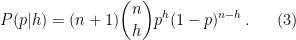
$\displaystyle P(p|h) = (n+1) \binom{n}{h} p^h(1-p)^{n-h} \,. \ \ \ \ \ (3)$

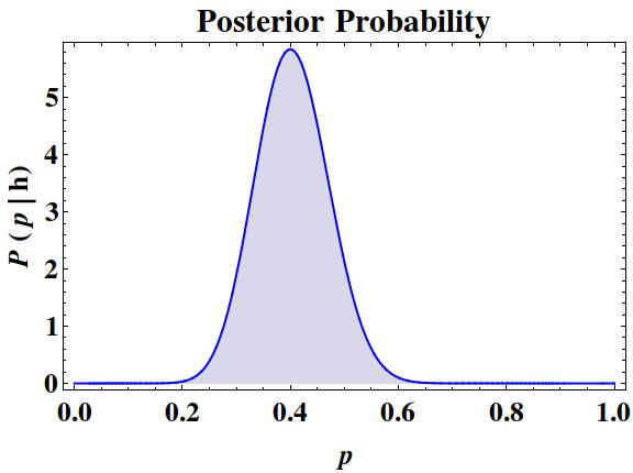
This looks like a binomial distribution but ${h}$ is fixed here and ${p}$ is the random variable. It is a beta distribution, conjugate to the binomial distribution.

The figure below shows the posterior probability $P(p|h)$ for h=20 and n=50. It peaks at $p=h/n=0.4$, the mode; the mean is $\bar p=(h+1)/(n+2)$ .

The posterior probability P(p|h) for h=20 and n=50.

A Limiting Case

Before getting to the odds, we look briefly at a limiting case. Suppose we “know” a priori that the coin is fair (this is unrealistic but instructive). Then we must choose ${P(p)=\delta(p-\frac{1}{2})}$ . The integral in the demominator of (2) is ${P(h|\frac{1}{2})}$ , so

$\displaystyle P(p | h) = \displaystyle{\frac{P(h|p)}{P(h|\frac{1}{2})}}\delta(p-\frac{1}{2}) = \delta(p-\frac{1}{2}) = P(p) \,,$

that is, the posterior probability is identical to the prior. Since we are certain from the outset, no amount of additional data can sway our conviction. But this never happens: no coin, however carefully minted, is guaranteed to be completely fair. In reality, we should consider a prior peaking sharply at ${p=\frac{1}{2}}$ rather than a delta-function. New information can then result in a change in the expected value of ${p}$ .

How Many Tosses?

The question raised above was how many tosses are needed to estimate the odds. Of course, this depends on the level of precision required. The posterior distribution for ${p}$ given ${h}$ is the beta distribution

$P(p|h) = (n+1) \binom{n}{h} p^h(1-p)^{n-h} \,.$

This is a standard beta distribution. The expected value of ${p}$ is

$\displaystyle E(p) \equiv \bar p = \frac{h+1}{n+2}$

and its variance is

$\displaystyle \mathrm{Var}(p) \equiv \sigma_p^2 = \frac{(h+1)(n-h+1)}{(n+2)^2(n+3)} = \frac{\bar p(1-\bar p)}{n+3}$

For large ${h}$ and ${n}$ we can write

$\displaystyle \bar p \approx \frac{h}{n} \qquad\mbox{and}\qquad \sigma_p \approx \sqrt{\frac{\bar p(1-\bar p)}{n}} \,.$

The quantity ${\sigma_p}$ is called the standard error.

We expect ${p}$ to be close to ${\bar p}$ , but we must be more specific. It is common to choose a confidence interval ${[\bar p-\kappa\sigma_p,\bar p+\kappa\sigma_p]}$ with ${\kappa=2}$ . For a normal distribution, this corresponds to 95% confidence: ${p}$ will be within this interval 95% of the time. We also specify a level of precision: let us require that ${p}$ differs from ${\bar p}$ by at most ${\epsilon}$ . To ensure this, we need

$\displaystyle \kappa\sigma_p = \kappa\sqrt{\frac{\bar p(1-\bar p)}{n}} < \epsilon \qquad\mbox{or}\qquad n > \kappa^2 \left[\frac{\bar p(1-\bar p)}{\epsilon^2}\right]$

Suppose the coin is approximately fair. Then ${\bar p\approx\frac{1}{2}}$ so ${\bar p(1-\bar p)\approx \frac{1}{4}}$ . If the confidence interval comprises values within two standard errors ( ${\kappa=2}$ ) and we require an accuracy of three significant figures ( ${\epsilon = 10^{-3}}$ ) then

$\displaystyle n > 4 \left(\frac{ \frac{1}{4} }{10^{-6}} \right) = 10^6 \,.$

This is amazing: we need on the order of a million tosses to have confidence in the estimated value of ${p}$ to three significant figures.

If we ask for six-figure accuracy, we need a trillion tosses!

Sources

Sharon Bertsch McGrayne, 2011: The Theory that would not Die. Yale Univ. Press, 336pp.

ThatsMaths