ToplDice is Markovian

Many problems in probability are solved by assuming independence of separate experiments. When we toss a coin, it is assumed that the outcome does not depend on the results of previous tosses. Similarly, each cast of a die is assumed to be independent of previous casts.

However, this assumption is frequently invalid. Draw a card from a shuffled deck and reveal it. Then place it on the bottom and draw another card. The odds have changed: if the first card was an ace, the chances that the second is also an ace have diminished.

Andrei Andreevich Markov

Andrei Andreevich Markov developed the theory of systems where the probability of the next outcome depends on the present state. He analysed a long poem of Alexander Pushkin, studying the patterns of vowels and consonants.

For the Roman alphabet there are five vowels and twenty-one consonants. If letters occurred randomly, the proportion of vowels in a long text would be 5/26, about a fifth, and the proportion of consonants would be 21/26 or about four fifths. However, the structure of language is not random. There is a strong tendency for vowels to be followed by consonants and vice versa.

A Markov chain is a process where the probabilities for the next outcome depend on the present state. The weather provides a simple example. Let us define some threshold to distinguish between hot and cold days. Due to the persistence of weather patterns, with warm spells and cool spells, a hot day is more likely than a cold day to occur tomorrow if today is hot. The probabilities for tomorrow’s weather depend on today’s weather.

ToplDice is a Markov Chain

Let’s consider a simple game, which we call Topple-Dice or ToplDice. A die is thrown randomly. The odds of any number from 1 to 6 are equal, at 1/6 or about 0.16667. However, instead of throwing the die again, we topple it through ninety degrees, choosing any of the four possible directions randomly.

Each number on the die is opposite its 7s-compliment: the numbers on opposite faces add to 7. Clearly, a 1 cannot become a 6 in one topple. Likewise, it cannot remain a 1. The other four possibilities ${\{2, 3, 4, 5 \}}$ are equally likely. In the same way, 3 and 4 cannot occur consecutively, nor can 2 and 5.

Let’s define the current state by a vector ${\mathbf{P}^{(n)} = (p_1, p_2, p_3, p_4, p_5, p_6)^\prime}$ . Then the transition matrix ${\boldsymbol{\mathsf{T}}}$ gives the probabilities for changes in one topple. Thus we have

$\displaystyle \mathbf{P}^{(n+1)} = \boldsymbol{\mathsf{T}} \mathbf{P}^{(n)} \,.$

The transition matrix is easily seen to be

$\displaystyle \boldsymbol{\mathsf{T}} = \begin{bmatrix} 0 & \frac{1}{4} & \frac{1}{4} & \frac{1}{4} & \frac{1}{4} & 0 \\ \frac{1}{4} & 0 & \frac{1}{4} & \frac{1}{4} & 0 & \frac{1}{4} \\ \frac{1}{4} & \frac{1}{4} & 0 & 0 & \frac{1}{4} & \frac{1}{4} \\ \frac{1}{4} & \frac{1}{4} & 0 & 0 & \frac{1}{4} & \frac{1}{4} \\ \frac{1}{4} & 0 & \frac{1}{4} & \frac{1}{4} & 0 & \frac{1}{4} \\ 0 & \frac{1}{4} & \frac{1}{4} & \frac{1}{4} & \frac{1}{4} & 0 \end{bmatrix}$

What happens after two topples? We square the transition matrix to get

$\displaystyle \boldsymbol{\mathsf{T}^2} = \begin{bmatrix} \frac{1}{4} & \frac{1}{8} & \frac{1}{8} & \frac{1}{8} & \frac{1}{8} & \frac{1}{4} \\ \frac{1}{8} & \frac{1}{4} & \frac{1}{8} & \frac{1}{8} & \frac{1}{4} & \frac{1}{8} \\ \frac{1}{8} & \frac{1}{8} & \frac{1}{4} & \frac{1}{4} & \frac{1}{8} & \frac{1}{8} \\ \frac{1}{8} & \frac{1}{8} & \frac{1}{4} & \frac{1}{4} & \frac{1}{8} & \frac{1}{8} \\ \frac{1}{8} & \frac{1}{4} & \frac{1}{8} & \frac{1}{8} & \frac{1}{4} & \frac{1}{8} \\ \frac{1}{4} & \frac{1}{8} & \frac{1}{8} & \frac{1}{8} & \frac{1}{8} & \frac{1}{4} \end{bmatrix}$

What about the long-term behaviour. Manual calculation is tedious, but we can easily calculate higher powers using a computer. For example, for 8 topples, the power of the transition matrix is

$\displaystyle \boldsymbol{\mathsf{T}^{8}} = \begin{bmatrix} 0.167969 & 0.166016 & 0.166016 & 0.166016 & 0.166016 & 0.167969 \\ 0.166016 & 0.167969 & 0.166016 & 0.166016 & 0.167969 & 0.166016 \\ 0.166016 & 0.166016 & 0.167969 & 0.167969 & 0.166016 & 0.166016 \\ 0.166016 & 0.166016 & 0.167969 & 0.167969 & 0.166016 & 0.166016 \\ 0.166016 & 0.167969 & 0.166016 & 0.166016 & 0.167969 & 0.166016 \\ 0.167969 & 0.166016 & 0.166016 & 0.166016 & 0.166016 & 0.167969 \end{bmatrix}$

We see that for ${n=8}$ the elements of the matrix are all about ${1.67}$ . For ${n=20}$ , the power of the transition matrix is

$\displaystyle \boldsymbol{\mathsf{T}^{20}} = \begin{bmatrix} 0.166667 & 0.166667 & 0.166667 & 0.166667 & 0.166667 & 0.166667 \\ 0.166667 & 0.166667 & 0.166667 & 0.166667 & 0.166667 & 0.166667 \\ 0.166667 & 0.166667 & 0.166667 & 0.166667 & 0.166667 & 0.166667 \\ 0.166667 & 0.166667 & 0.166667 & 0.166667 & 0.166667 & 0.166667 \\ 0.166667 & 0.166667 & 0.166667 & 0.166667 & 0.166667 & 0.166667 \\ 0.166667 & 0.166667 & 0.166667 & 0.166667 & 0.166667 & 0.166667 \end{bmatrix}$

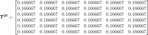
Clearly, it has converged to ${\frac{1}{6}\boldsymbol{\mathsf{E}}}$ , where ${\boldsymbol{\mathsf{E}}}$ is the matrix with all elements equal to unity. This implies that, in the long term, all six numbers of the die are equally likely to show up.

For weather forecasts, this is easily understood. A hot day today may tell us something about the likelihood of hot weather tomorrow, but it doesn’t tell us anything about the weather one year ahead. For that, we have to resort to climatological statistics.

Markov chains are now used to analyse very large systems with thousands of variables. They are at the heart of Bayesian statistical analysis. The modern explosion of computer power has enabled us to obtain solutions to problems that were beyond our dreams until recently.

See earlier post on this blog, here.

Related

Published by thatsmaths