Circles, polygons and the Kepler-Bouwkamp constant

If circles are drawn in and around an equilateral triangle (a regular trigon), the ratio of the radii is ${\cos \pi/3 = 0.5}$ . More generally, for an N-gon the ratio is easily shown to be ${\cos \pi/N}$ . Johannes Kepler, in developing his amazing polyhedral model of the solar system, started by considering circular orbits separated by regular polygons (see earlier post on the Mysterium Cosmographicum here).

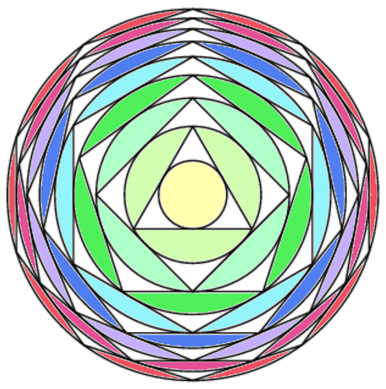
Kepler was unable to construct an accurate model using polygons, but he noted that, if successive polygons with an increasing number of sides were inscribed within circles, the ratio did not diminish indefinitely but appeared to tend towards some limiting value. Likewise, if the polygons are circumscribed, forming successively larger circles (see Figure below), the ratio tends towards the inverse of this limit. It is only relatively recently that the limit, now known as the Kepler-Bouwkamp constant, has been established.

Let us start with the unit circle, and draw a nested sequence of regular polygons, of increasing order and size, each with its circumcircle (see Figure). Thus, we have a trigon (triangle), a tetragon (square), a pentagon, a hexagon, and so on to the N-gon. The outermost circle, surrounding the N-gon, has radius

$\displaystyle R = \left[ \cos\frac{\pi}{3} \times \cos\frac{\pi}{4} \times \cos\frac{\pi}{5} \times \cdots \times \cos\frac{\pi}{N} \right]^{-1} \,. \ \ \ \ \ (1)$

In their popular book Mathematics and the Imagination, Edward Kasner and James Newman described this problem and stated that the limit of ${R}$ is approximately equal to 12. They gave no indication of the source of this estimate. In 1965, C J Bouwkamp showed that the true value is much smaller:

$\displaystyle R = 8.700\,036\,625\,208\,194\,5 \dots \qquad (2)$

Moving inwards instead of outwards, the ratio of the inscribed and circumscribed circles for an N-gon is again ${\cos \pi/N}$ , so the radius of the innermost circle is

$\displaystyle \rho = \cos\frac{\pi}{3} \times \cos\frac{\pi}{4} \times \cos\frac{\pi}{5} \times \cdots \times \cos\frac{\pi}{N} \,.$

The infinite product

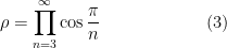
$\displaystyle \rho = \prod_{n=3}^\infty \cos\frac{\pi}{n} \qquad\qquad\qquad (3)$

is very slowly converging. Bouwkamp gave the following estimate for this constant:

$\displaystyle \rho = 0.114\,942\,044\,853\,296\,2 \dots \qquad (4)$

Bouwkamp remarked that there was no known closed expression for ${\rho}$ , and that he did not expect that any such expression existed. He developed two methods for evaluating the constant. They involved the Riemann zeta function, for which tables of values were available.

Today, it is a simple matter to evaluate ${R}$ and ${\rho}$ using a mathematical computing system like Mathematica. In the Figure above, we show the value of the finite approximants to the product (3) for a range of ${N}$ up to 10,000. For ${N=100}$ , we get ${R = 8.287}$ with only one correct digit. When ${N=1000}$ , we get ${R=8.657}$ with two accurate digits. The values produced for the extreme value ${N=10\,000}$ are

$\displaystyle R \approx 8.695\,745\,031\,934\,219\,2 \quad\mbox{and}\quad \rho \approx 0.114\,998\,771\,965\,783\,7$

From these results, we see the painfully slow rate of convergence. Comparing with (2) and (4), even with 10,000 terms, we have only a few digits accuracy. Bouwkamp’s formula yields far more accurate estimates.

Sources

${\bullet}$ Bouwkamp, C. J., 1965: An infinite product. Indagationes Mathematic\ae, 68, 40–46.

${\bullet}$ Kasner, Edward and James Newman, 1940: Mathematics and the Imagination. Reprinted by Dover Books, 2000.

${\bullet}$ Wikipedia article: Kepler-Bouwkamp constant. http://www.wikipedia.org/

Related

Published by thatsmaths