We are all familiar with simple mathematical puzzles that give a short sequence and ask “What is the next number in the sequence”. Simple examples would be
the sequence of odd numbers, the sequence of squares and the Fibonacci sequence.
The Pitfalls of Generalising
Circle division: points, chords, regions.
The idea is to spot the rule by which the terms of the sequence are generated. But the rule is never really determined by the first few terms, so the answer is not unique. Indeed, it is simple to construct a rule that matches the given terms and also generates an arbitrary value for the next term.
Let us ask “How many regions are formed if each of a set of points on a circle is joined by a chord to all the other points?” (see figure). For small it is easy to count the regions. It is tempting to assume that the sequence, which begins reveals the general pattern for all values of But this formula breaks down for , when there are 31 regions. Thus, we may argue that the next number in the sequence is 31.
Lagrange Polynomials
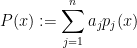
Suppose the given terms are . Linderholm (1971), in his light-hearted book “Mathematics Made Difficult”, argued that we can define a polynomial that passes through all the points and also through an arbitrary value. We first define the polynomial
For , we have , and for we have . Now defining
we see that for , so the polynomial interpolates between the given terms .
Now we extend the definitions to include an extra term:
and
Then for and . Using the polynomial we can argue that the next term in the sequence can take any randomly chosen value .
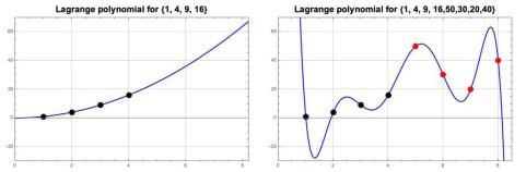
In the figure below (left panel) we plot the sequence and the interpolating polynomial that fits all four points.
Then we extend the sequence in an arbitrary fashion, say , and plot the interpolating polynomial that fits all eight points:
The result is shown in the figure (right panel).
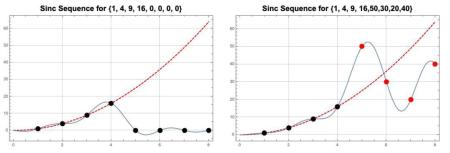
Sinc Sequences
The sinc function is defined thus:
We note that oscillates with decaying amplitude as increases, and has zeros at . Thus, the function equals for and is zero for all other integer values of . It is clear that, given a finite sequence , the function
takes the values of the sequence at . We can extend the sequence by appending an arbitrary value, , and we can define an interpolating function that takes the values at :
Using , we can argue that is the “natural next number” in the sequence .
For example, we plot the sequence and the sinc expansion that fits all four points (left panel in figure below). Then we extend the sequence arbitrarily to and plot the corresponding sinc sum (right panel).
Conclusion
Given the initial terms of a sequence, there are many ways to define a function that fits all the given values and also takes arbitrary subsequent values. This, in purely logical terms, the question “What is the next Number?” does not have a well-defined answer. However, if you apply this logic in your MCQ or your IQ test, you may score badly.
Sources
Linderholm, Carl E., 1971: Mathematics Made Difficult. Wolfe Publishing, London. 207 pages SBN: 72340415 1.

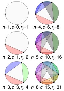
 points,
  chords,
  regions.


![\displaystyle \hat f_n(x) = \sum_{k=1}^{n} [ a_k\,\mathrm{sinc\ }\pi(x-k) ] + A\,\mathrm{sinc\ }\pi(x-(n+1)) \,.](https://s0.wp.com/latex.php?latex=%5Cdisplaystyle+%5Chat+f_n%28x%29+%3D+%5Csum_%7Bk%3D1%7D%5E%7Bn%7D+%5B+a_k%5C%2C%5Cmathrm%7Bsinc%5C+%7D%5Cpi%28x-k%29+%5D+%2B+A%5C%2C%5Cmathrm%7Bsinc%5C+%7D%5Cpi%28x-%28n%2B1%29%29+%5C%2C.+&bg=ffffff&fg=000000&s=0&c=20201002)