Curvature and the Osculating Circle

Curvature is of critical importance in numerous contexts. An example is shown in the figure above, a map of the Silverstone Formula 1 racetrack. The sharp bends (high curvature) force drivers to reduct speed drastically.

The Concept of Curvature

Curvature is a fundamental concept in differential geometry. The curvature of a plane curve is a measure of how much it deviates from a straight line. We can compute the curvature as the limit of the angle through which the tangent at a point turns as the point moves through a small distance along the curve.

The simplest example of a curve is a circle. As a point moves around a circle, the tangent curve turns through a full rotation. Thus, the curvature is

$\displaystyle \kappa = \frac{\mbox{Change of Direction}}{\mbox{Distance Travelled}} = \frac{2\pi}{2\pi R} = \frac{1}{R} \,.$

Thus, a circle has curvature equal to the reciprocal of the radius. A straight line is the limiting case of a circle as the radius becomes infinite, and the curvature tends to zero.

In general, the curvature of a differentiable curve at a point is the curvature of the circle that most closely approximates the curve near the point, the so-called osculating circle. We can choose three points on the curve and determine the circle that passes through them. As the three points coallesce to a single point, this circle becomes the osculating circle, and its radius determines the curvature at the point.

Direct Calculation of Curvature

Fig. 1. Changing slopes between points on ${y=f(x)}$ .

We evaluate a function ${y = f(x)}$ at point ${P_2=(x_2,y_2)}$ and at two neighbouring ${P_1=(x_1,y_1)}$ and ${P_3=(x_3,y_3)}$ where ${x_1 = x_2 - \Delta x}$ and ${x_3 = x_2 + \Delta x}$ (see Fig. 1). We define the mean gradients

$\displaystyle m_{12} = \frac{y_2-y_1}{\Delta x} \,, \qquad m_{23} = \frac{y_3-y_2}{\Delta x} \,.$

The second derivative at ${x_2}$ is

$\displaystyle y_2^{\prime\prime} \approx \frac{m_{23}-m_{12}}{\Delta x} \ \ \ \ \ (1)$

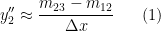
The tangent angles over the intervals ${[x_1,x_2]}$ and ${[x_2,x_3]}$ are

$\displaystyle \theta_1 = \arctan m_{12} \qquad \theta_2 = \arctan m_{23}$

Then using a standard result for the difference of two arc-tangents,

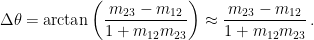
$\displaystyle \Delta\theta = \arctan\left(\frac{m_{23}-m_{12}}{1+m_{12}m_{23}}\right) \approx \frac{m_{23}-m_{12}}{1+m_{12}m_{23}} \,.$

Using (1) and approximating ${m_{12}}$ and ${m_{23}}$ by ${m_2}$ ,

$\displaystyle \Delta\theta \approx \frac{y_2^{\prime\prime}\Delta x}{1+m_2^2}$

The arc-length between the midpoints of ${[x_1,x_2]}$ and ${[x_2,x_3]}$ is

$\displaystyle \Delta s^2 \approx \Delta x^2 (1 + m_2^2) \,.$

Combining the above two equations, the curvature is

$\displaystyle \kappa \approx \frac{\Delta\theta}{\Delta s} \approx \frac{y_2^{\prime\prime}}{(1+m_2^2)^{3/2}} \,. \ \ \ \ \ (2)$

The Osculating Circle

We can derive an expression for the osculating circle at ${P}$ by taking three points close to ${P}$ . First, let us consider three general points, ${(x_1,y_1)}$ , ${(x_2,y_2)}$ , and ${(x_3,y_3)}$ . Suppose the circle passing through these three points has centre at ${(x_c,y_c)}$ , and radius ${R}$ . Then

$\displaystyle (x_1 - x_c )^2 + ( y_1 - y_c)^2 = R^2 \ \ \ \ \ (3)$
$\displaystyle (x_2 - x_c )^2 + ( y_2 - y_c)^2= R^2 \ \ \ \ \ (4)$
$\displaystyle (x_3 - x_c )^2 + ( y_3 - y_c)^2 = R^2 \ \ \ \ \ (5)$

These are three quadratic equations for three unknowns, ${\{x_c, y_c, R \}}$ . We can get two linear equations for ${\{x_c, y_c \}}$ by subtracting (3) from (4) and (4) from (5) and rearranging:

$\displaystyle 2 (x_2-x_1) x_c + 2 (y_2-y_1) y_c = (x_2^2-x_1^2) + ( y_2^2-y_1^2) \ \ \ \ \ (6)$
$\displaystyle 2 (x_3-x_2) x_c + 2 (y_3-y_2) y_c = (x_3^2-x_2^2) + ( y_3^2-y_2^2) \ \ \ \ \ (7)$

We can easily solve these simultaneous linear equations for ${(x_c, y_c)}$ , the centre of the circle. Then any one of the equations (3)–(5) can be used to find the radius ${R}$ (see Fig. 2, left panel).

Coalescing Points

The curvature of the graph of a function ${y = f(x)}$ at a point ${P}$ with coordinates ${(x_0,y_0)}$ depends on the second derivative ${y^{\prime\prime} = \mathrm{d}^2 f/ \mathrm{d}x^2}$ . But what is the precise relationship?

Let us suppose that the three points are close together, and expand to second order:

$\displaystyle \begin{array}{rcl} x_1 = x_2 - \Delta x &\quad& y_1 = y_2 - y_2^\prime \Delta x + \textstyle{\frac{1}{2}} y_2^{\prime\prime} \Delta x^2 \\ x_3 = x_2 + \Delta x &\quad& y_3 = y_2 + y_2^\prime \Delta x + \textstyle{\frac{1}{2}} y_2^{\prime\prime} \Delta x^2 \end{array}$

Therefore, to second order, we get

$\displaystyle \begin{array}{rcl} (x_2^2 - x_1^2) = 2x_2\Delta x - \Delta x^2 &\quad& (y_2^2 - y_1^2) = +(2 y_2 y_2^\prime)\Delta x - ( y_2^{\prime 2} - y_2y_2^{\prime\prime}) \Delta x^2 \\ (x_3^2 - x_2^2) = 2x_2\Delta x + \Delta x^2 &\quad& (y_2^2 - y_1^2) = -(2 y_2 y_2^\prime)\Delta x - ( y_2^{\prime 2} - y_2y_2^{\prime\prime}) \Delta x^2 \end{array}$

Fig. 2. Left: circle through three points on the curve. Right: osculating circle through three `coalescing’ points.

To simplify matters, let us assume the origin is moved to the point ${(x_2, y_2)}$ and the ${x}$ -values are equally spaced: ${x_1 = -\Delta x}$ and ${x_3 = +\Delta x}$ (see Fig. 2, right panel). Expanding to order ${\Delta x^2}$ we have

$\displaystyle y_1 = -y_2^\prime \Delta x + \textstyle{\frac{1}{2}} y_2^{\prime\prime} \Delta x^2 \,, \qquad y_3 = \phantom{+}y_2^\prime \Delta x + \textstyle{\frac{1}{2}} y_2^{\prime\prime} \Delta x^2 \,,$

or, defining ${m = y_2^\prime}$ and ${\gamma = y_2^{\prime\prime}}$ ,

$\displaystyle \begin{array}{rcl} y_1 &= -m \Delta x + \textstyle{\frac{1}{2}}\gamma \Delta x^2 \,,\qquad y_1^2 &= m^2 \Delta x^2 \\ y_3 &= \phantom{+}m \Delta x + \textstyle{\frac{1}{2}} \gamma \Delta x^2 \,,\qquad y_3^2 &= m^2 \Delta x^2 \end{array}$

Using these in (6) and (7) and subtracing one from the other, gives

$\displaystyle y_c = (1 + m^2) / \gamma$

Adding the two gives

$\displaystyle 2 x_c + 2 m y_c = 0 \qquad\mbox{or}\qquad x_c = - m y_c \,.$

Now we can compute ${R^2}$ :

$\displaystyle R^2 = x_c^2 + y_c^2 = (1+m^2)[(1+m^2)^2 / \gamma^2] \,.$

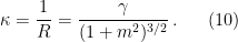
Finally, recalling that ${\gamma = y_2^{\prime\prime}}$ , we get the expression for curvature,

$\displaystyle \kappa = \frac{1}{R} = \frac{\gamma} {(1+m^2)^{3/2} } \,. \ \ \ \ \ (10)$

which agrees with (2).

Curvature in Higher Dimensions

The curvature of a two-dimensional surface is a measure of how much it deviates from a plane. More generally, for a Riemannian manifold of dimension ${n}$ we can define the curvature intrinsically, that is without considering the embedding in an external space. This is done by means of the Riemann curvature tensor. For a two-dimensional surface, we can define the maximal curvature, minimal curvature, and mean curvature.

Much more can be written about the topic of curvature. The Wikipedia article Curvature is an excellent place to begin deeper investigations.

ThatsMaths