Vertical or Horizontal Slices? Riemann and Lebesgue Integration.

For simple sets, we have geometric length, area and volume. But how can we establish these dimensions for complicated curves, areas and volumes. Integral calculus provides a powerful tool for answering such questions. The area ${A}$ between the curve ${y=y(x)}$ and the ${x}$ -axis is

$\displaystyle A = \int_{x_1}^{x_2} y(x) \mathrm{dx} \,.$

The usual definition of an integral, following Bernhard Riemann, works fine for reasonably well-behaved functions over finite intervals.

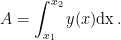
Chopping into Vertical Slices

We briefly recall the definition of the Riemann integral. Consider on the finite interval ${[a, b] \subset \mathbb{R}}$ , the set of points

$\displaystyle \pi := \{a = t_0 , t_o+\Delta t, t_0+2\Delta t, \dots , t_0+ k \Delta t = t_N = b \} \,.$

For a function ${f : [a, b] \rightarrow \mathbb{R}}$ , we define

$\displaystyle m_j = \inf_{t \in [t_{j-1},t_j]} f(t) \,, \quad M_j = \sup_{t \in [t_{j-1},t_j]} f(t) \,, \quad j = 1, 2, \dots , N \,.$

We introduce the lower and upper Darboux sums

$\displaystyle S_{\pi}[f] := \sum_{j=1}^N m_j \Delta t \qquad\mbox{and}\qquad S^{\pi}[f] := \sum_{j=1}^N M_j \Delta t$

A bounded function ${f : [a, b] \rightarrow \mathbb{R}}$ is Riemann integrable if the quantities

$\displaystyle \int_{*} f := \sup_{\pi} S_{\pi}[f] \qquad\mbox{and}\qquad \int^{*} f := \inf_{\pi} S^{\pi}[f]$

are finite and have the same value. This common value is called the Riemann integral of ${f}$ and denoted by ${\int_a^b f(t)\,\mathrm{d}t}$ .
But what if the function to be integrated is wild in some way, or the region over which it is to be integrated is complicated? For example, the characteristic function, or indicator function, of the set of rational numbers in the interval ${[0,1]}$ equals 1 for rationals and 0 for irrationals. It oscillates between these values an infinite number of times within any interval, however small, so that the upper and lower Darboux sums never converge.

Slicing up an area for Riemann integration (left panel) and Lebesgue integration (right panel) [Figures from Schilling (2005)].

The reason for the difficulty is that the Riemann sums partition the domain of the function without taking into account the shape of the function, thus slicing up the area under the function vertically (Figure above, left panel).

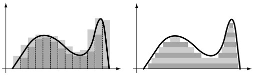
Chopping into Horizontal Slices

Lebesgue’s approach to integration is in sharp contrast to Riemann’s: the domain is partitioned according to the values of the function under consideration, resulting in a decomposition of the area into horizontal slices (Figure above, right panel).

The set of functions that are Lebesgue integrable is substantially greater than the set of Riemann integrable functions. For example, the set of rational numbers in the interval ${[0,1]}$ has Lebesgue measure 0; the set of irrational numbers in this interval has measure 1. Thus, informally, there are “many more” irrationals than rationals. This concurs with the cardinality of these sets (although this concurrence is not guaranteed in general).

While the scope of measure theory is much broader than Riemann’s integral, it is impossible to define a functional that yields an integral for every function: there are always functions that cannot be integrated and sets that cannot be measured.

The good news is that, for most `well-behaved’ functions, the Riemann and Lebesgue integrals both exist and both have the same value.

Conclusions

The Riemann integral is convenient for calculating the primitive, or anti-derivative, of the integrand of `reasonably behaved’ functions. However, it fails to provide a meaningful results for more exotic functions. The Lebesgue theory comes to the rescue, and it provides very powerful theorems that justify the interchange of limits and integrals.

Sources
${\bullet}$ Schilling, René L., 2005: Measures, Integrals and Martingales. Cambridge Univ. Press, 381pp. ISBN 978-0-5216-1525-9.

${\bullet}$ Wikipedia articles: (1) Riemann Integral. (2) Lebesgue integration.

Related

Published by thatsmaths