Predator-Prey Models

Next week’s post will be about a model of the future of civilization! It is based on the classical predator-prey model, which is reviewed here.

Solution for X(T) and Y(T) for 30 time units. X(0)=0.5, Y(0)=0.2 and k=0.5.

Solution for X (blue) and Y (red) for 30 time units. X(0)=0.5, Y(0)=0.2 and k=0.5.

The Lotka-Volterra Model

Many ecological process can be modelled by simple systems of equations. An early example of this is the predator-prey model, developed independently by American mathematician Alfred Lotka (1880–1949) and Italian Vito Volterra (1860-1940).

The interaction between two species of animals, one preying on the other, can be simulated by two first-order nonlinear ordinary differential equations. As an example, we consider rabbits as prey and foxes as predators. Letting ${x}$ be the number of rabbits and ${y}$ the number of foxes, the rates of change of the two populations are given by

$\displaystyle \frac{dx}{dt} = (\alpha - \beta y) x \qquad\qquad \frac{dy}{dt} = -(\gamma - \delta x) y$

These are the Lotka-Volterra equations. Of their nature, ${x}$ and ${y}$ are positive quantities. We also assume that all the parameters are positive. Parameters ${\alpha}$ and ${\gamma}$ are the reproduction rates. If only rabbits are present ( $x>0, y=0$ ) their exponential growth is determined by ${\alpha}$ . If there are only foxes ( ${x=0,y>0}$ ), they die out at a rate determined by ${\gamma}$ , as there is no food available to them. When both species are present, ${\beta}$ and ${\delta}$ determine the interaction between them.

The equation for the prey ${x}$ says that the change in population is determined by the growth rate ${\alpha}$ minus the predation rate ${\beta y}$ . For the predators, the second equation says that their population is determined by the food supply ${\delta x}$ minus their natural death rate ${\gamma}$ .

Scaling and Solution

We can re-scale ${x}$ , ${y}$ and the time ${t}$ so that the system depends on a single parameter. Let ${X = \delta x/\gamma}$ , ${Y = \beta y/\alpha}$ and ${T = \alpha t}$ . Then we get the canonical form

$\displaystyle \frac{dX}{dT} = (1 - Y) X \qquad\qquad \frac{dY}{dT} = - k(1 - X) Y$

where ${k=\gamma/\alpha}$ . The right hand sides give the velocity in phase space:

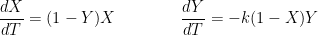
$\displaystyle \mathbf{V} \equiv (X^\prime, Y^\prime) = ( X - XY , kXY -kX )$

In Fig. 1 we plot the velocity in the ${(X,Y)}$ phase-plane for the case ${k=1}$ .

Phase-space for the Lotka-Volterra equations.

Fig. 1. Velocity field for the Lotka-Volterra equations with k=1. Prey on X-axis and predators on Y-axis.

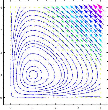
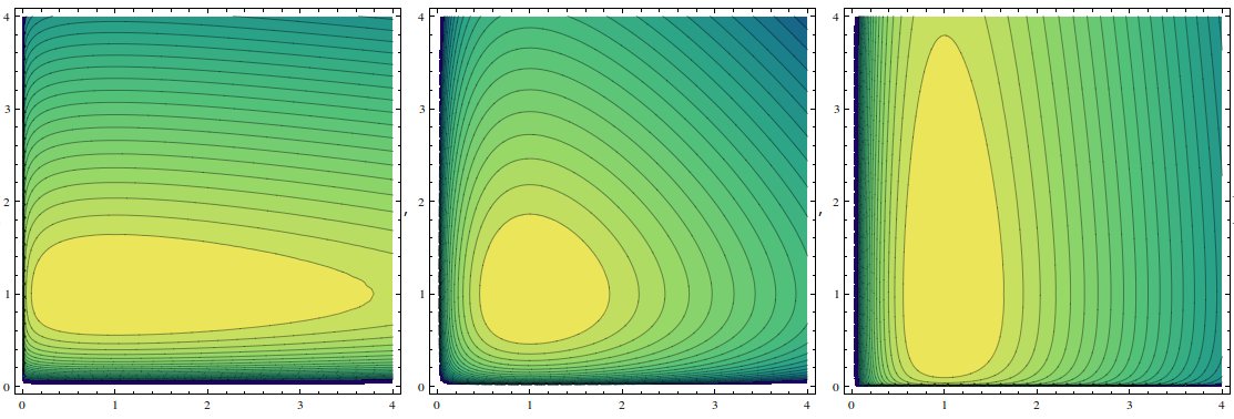
Although the equations are nonlinear, they can be solved. Taking the ratio of the two equations, we get a separable equation which can be integrated immediately to yield a constant quantity:

$\displaystyle Z(k) \equiv k\log X + \log Y - (kX + Y) = \mathrm{Const.}$

Fig. 2 shows the contours of ${Z(k)}$ for three values of the parameter ${k}$ . It is clear that both ${X}$ and ${Y}$ vary periodically, but out of phase. The phase-point traces out a contour in an anti-clockwise direction, with ${Y}$ lagging about a quarter-cycle behind ${X}$ . First, the rabbits increase in number. The extra food allows fox numbers to grow. But as predation increases, rabbit numbers fall leading to reduced food for the foxes, which decline in numbers.