New Curves for Old: Inversion

Special Curves

A large number of curves, called special curves, have been studied by mathematicians. A curve is the path traced out by a point moving in space. To keep things simple, we assume that the point is confined to two-dimensional Euclidean space ${\mathbb{R}^2}$ so that it generates a plane curve as it moves. This, a curve results from a mapping ${\mathbf{\gamma} : [a,b]\longrightarrow \mathbb{R}^2}$ .

Special curves have played a central role in the development of mathematics. Seventeenth century mathematicians were interested in rectifying curves — that is, calculating their arc-lengths — and also finding the areas surrounded by closed curves. These questions stimulated the evolution of differential and integral calculus.

Simple Constraints

Many simple curves can be defined by applying simple constraints. If the generating point remains at a constant distance from a fixed point ${O}$ , a circle emerges. If it is equidistant from two fixed points, it traces a straight line. If the sum of the distances from two points ${O}$ and ${O^\prime}$ , called the foci, is constant, we get an ellipse. If the difference between these distances is constant, a hyperbola is generated. If the product of the two distances is constant, the result is a Cassinian oval. If the ratio is constant, the curve is a circle.

Inversion with respect to a circle

Given any plane curve ${\cal C}$ , we can generate a range of other curves. Examples are the evolute, the involute and the pedal curves. We consider here the curve that is the inverse of a given curve ${\cal C}$ with respect to a fixed point. To form the inverse, we specify a point ${O}$ called the centre of inversion, and the circle of unit radius centered at ${O}$ . To keep things simple, we take ${O}$ to be the origin. For each point ${(x,y)}$ on the curve ${\cal C}$ , we define an inverse point ${(x^\prime,y^\prime)}$ by

$\displaystyle x^\prime = \frac{x}{x^2+y^2} \,, \qquad y^\prime = \frac{y}{x^2+y^2} \,.$

It is clear that ${xx^\prime+yy^\prime=1}$ . The points ${(x,y)}$ and ${(x^\prime,y^\prime)}$ are on the same ray from ${O}$ , at distances ${r=\sqrt{x^2+y^2}}$ and ${r^\prime=\sqrt{{x^\prime}^2+{y^\prime}^2}}$ respectively, such that ${rr^\prime = 1}$ . If the inversion is applied twice, we recover the original point.

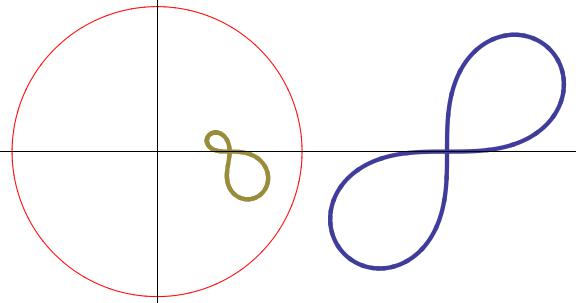
Lemniscate centred at (2,0 ) (blue) and its inverse (green) wrt the unit circle centred at the origin.

As the point ${(x,y)}$ moves along the curve ${\cal C}$ , the inverse points ${(x^\prime,y^\prime)}$ trace out the inverse curve ${\cal C^\prime}$ . If we replace the unit circle by a circle of radius ${k}$ , then the inverse point is such that ${rr^\prime=k^2}$ and the curve ${\cal C^\prime}$ has the same shape but is scaled by a factor ${k}$ .

In polar coordinates the inversion is especially simple. The inverse of the point ${(r,\theta)}$ with respect to the unit circle is ${(r^\prime,\theta^\prime)=(1/r,\theta)}$ . Thus, if the original curve ${\cal C}$ is expressed in the form ${r=f(\theta)}$ , the inverse curve ${\cal C^\prime}$ is ${r=1/f(\theta)}$ .

Simple examples of inverse curves

A line through the origin has polar equation ${\theta=\theta_0}$ and the inverse curve has the same equation, thus ${\cal{C}=\cal{C}^\prime}$ . An arbitrary line can be written ${r\cos(\theta-\theta_0)=a}$ , and its inverse is ${r = [\cos(\theta-\theta_0)]/a}$ . This is the equation of a circle passing through the origin. More generally, the inverse of a circle not passing through ${O}$ is another circle.

A conic section with focus at the origin has polar equation ${r = {1}/{(1+e\cos\theta)}}$ , so the inverse curve (wrt ${O}$ ) is given by ${r = {1+e\cos\theta}}$ . This is the limaçon of Pascal. For ${e=1}$ the conic is a parabola and the inverse is a special case of the limaçon called a cardioid. The three cases, ellipse ( ${e<1}$ ), parabola ( ${e=1}$ ) and hyperbola ( ${e>1}$ ) are shown in the figure below.

Conic sections (blue curves) and their inverses wrt the focus (green curves). Left: {e1}, hyperbola. The inverse curves are limaçons. For the parabola the inverse is a cardioid.

Conic sections (blue curves) and their inverses wrt the focus (green curves). Left: {e<1}, ellipse. Centre: {e=1} , parabola. Right: {e>1}, hyperbola. The inverse curves are limaçons. For the parabola the inverse is a cardioid.

Inverse of a rectangular hyperbola wrt its centre

The inverse changes with the point of inversion. We saw that a hyperbola wrt the focus is a limaçon. Now we look at the inverse wrt the centre. The usual equation for a hyperbola in cartesian coordinates is

$\displaystyle \frac{x^2}{a^2} - \frac{y^2}{b^2} = 1 \,.$

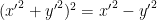
Taking ${a=b=1}$ and inverting with respect to the origin we get, after some juggling,

$\displaystyle ({x^\prime}^2+{y^\prime}^2)^2 = {x^\prime}^2-{y^\prime}^2$

which represents the lemniscate (lemniscus means a knotted ribbon), a figure-of-eight curve studied by Jakob Bernoulli in 1694. Bernoulli’s work on the arc length of the lemsnicate laid the foundation for later work on elliptic integrals and functions.

It is easier to work in polar coordinates. With ${x=r\cos\theta}$ and ${y=r\sin\theta}$ , the equation for the hyperbola (with ${a=b}$ ) is ${r^2\cos 2\theta = a^2}$ so the inverse may immediately be written ${r^2 = [\cos 2\theta]/a^2}$ . This converts back to the cartesian form given above.

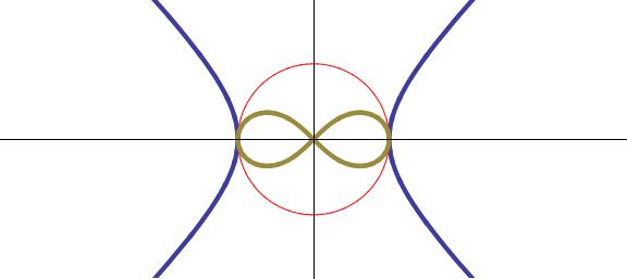
$Hyperbola {x^2-y^2=1} and its inverse {({x^\prime}^2+{y^\prime}^2)^2 = {x^\prime}^2-{y^\prime}^2}, the lemniscate of Bernoulli.$

Hyperbola x^2-y^2=1 and its inverse (x^2+y^2)^2 = x^2-y^2, the lemniscate of Bernoulli.

Inversion and the Riemann sphere

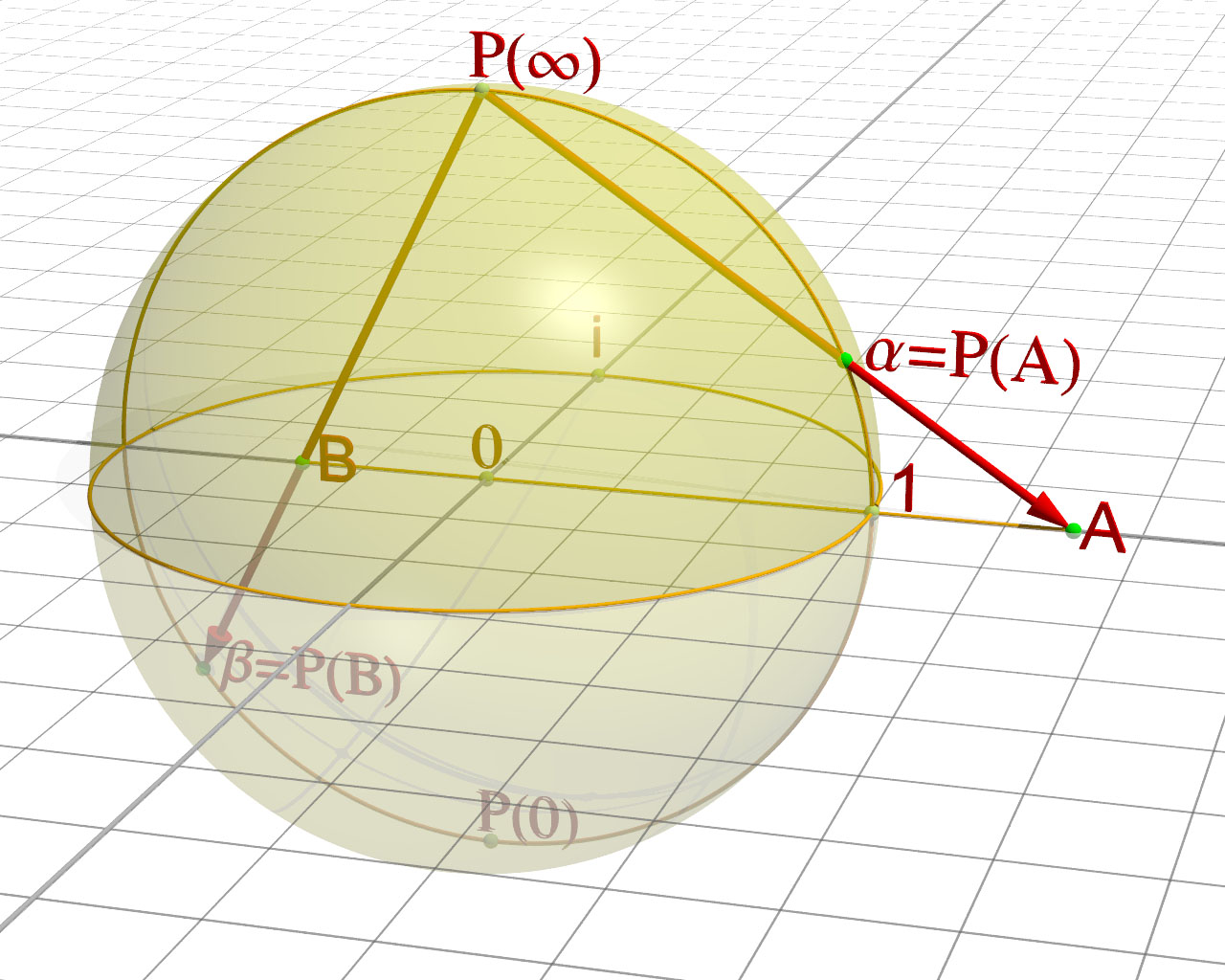
There is another way to view inversion — in mathematics, there is always another way! We can map the plane ${\mathbb{R}^2}$ onto the 2-sphere ${S^2}$ in ${\mathbb{R}^3}$ . ${S^2}$ is given by ${\{(x,y,z):x^2+y^2+z^2=1\}}$ . The map is a stereographic projection, as shown in the figure below. A line from the north pole ${(0,0,1)}$ links a point on the sphere to each point in the equatorial plane.

Stereographic mapping of the plane onto the Riemann sphere. Image: Jean-Christophe Benoist, Wikipedia.

Points on the sphere can be specified by co-latitude ${\theta}$ and longitude ${\phi}$ . The southern hemisphere ( ${\theta>\pi/2}$ ) maps to the interior of the unit circle in ${\mathbb{R}^2}$ . The northern hemisphere ( ${\theta<\pi/2}$ ) maps to the exterior. A point ${(\theta,\phi)}$ in ${S^2}$ maps onto the point in the plane ${\mathbb{R}^2}$ with polar coordinates ${(r,\phi)=(\cot\frac{\theta}{2},\phi)}$ .

Reflection in the equatorial plane ${(x,y,z)\longrightarrow(x,y,-z)}$ maps a point ${(\theta,\phi)}$ to ${(\theta^\prime,\phi^\prime)=(\pi-\theta,\phi)}$ . We easily show that ${(\theta^\prime,\phi^\prime)}$ maps under stereographic projection to ${(r^\prime,\phi^\prime)=(\tan\frac{\theta}{2},\phi)}$ . Therefore, ${rr^\prime = 1}$ , so reflection in ${S^2}$ corresponds to inversion in ${\mathbb{R}^2}$ .

* * * * * *

Looking for the ideal Christmas present? Look no further:

Peter Lynch’s book about walking around the coastal counties of Ireland is now available as an ebook (at a very low price!). For more information and photographs go to http://www.ramblingroundireland.com/

ThatsMaths